Mathematica Eterna
Open Access

Stochastic Characterization and Numerical Analysis of Prime Gaps for Stationary Distribution Approximation

George Gabriel^{* *}Correspondence: George Gabriel, Department of Mathematics and Statistics, McGill University, Quebec, Canada, Email:

Author info »

Introduction

Prime gaps have been the subject of mathematical inquiry for centuries, with early contributions from Euclid to more recent advancements by mathematicians such as Hardy et al., Erdos [1- 3]. Recent breakthroughs by Goldston et al., Zhang, have provided new impetus to this field of study [4,5]. The prime number theorem, which approximates the distribution of primes, suggests that primes become less frequent as numbers increase, yet does not fully explain the variability in the gaps between consecutive primes [6].

The distribution of prime gaps is conjectured to follow certain probabilistic models, including poisson-like distributions for larger gaps. The Hardy et al., conjectures, specifically the first conjecture, predict the density of prime pairs separated by a specific even gap, proposing that the occurrence of such pairs can be modelled by a non-trivial multiplicative function over the primes [2]. This study leveraged the computational resources of the Canadian supercomputer “Béluga” to perform large-scale calculations, generating up to 10¹² prime gaps using the Sieve of Eratosthenes algorithm. This extensive dataset was crucial in validating the accuracy and robustness of the models developed in this research.

Materials and Methods

Stochastic modeling of prime gaps using Markov chains

A discrete time Markov chain

is a stochastic process with states S = {j: j∈Z} indexed by discrete time T such that:

In the context of a Markov chain, the transition matrix P is a matrix that describes the probabilities of transitioning from one state to another. Each entry P_ij in the transition matrix represents the probability of moving from state i to state j in one step.

The probability

is denoted by P_ij and the matrix P = (P_ij ) is called a one-step transition matrix. The matrix P is a stochastic matrix in the sense that:

Required to use P as a model for the sequence of prime gaps

is the n^-th prime number. Although primes are not random, their appearance in the number sequence is unpredictable and so, they are often modeled as random numbers. We remark that for small values of n, the model P is a poor representation of the behavior of prime gaps because the probability that the system is in state j at time n depends not only on the immediate past state i but also on the states before that down to the state at the 0^-th step. For moderate to large values of n, this dependence on the other past states disappears.

The limiting distribution of a Markov chain is a probability distribution that remains unchanged 2 as the chain evolves over time. It represents the long-term behavior of the system. Define

to be the marginal distribution of

be the row vector:

Then, mathematically, a Markov chain is said to have a limiting distribution if for all i, j ∈ S:

such that;

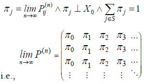
The stationary distribution is a special type of limiting distribution that satisfies the equation:

Indicating that once the system reaches this distribution, it remains there indefinitely. The stationary distribution can be interpreted as the equilibrium state of the Markov chain.

The relationship between the transition matrix, limiting distribution, and stationary distribution is important for understanding the long-term behavior of the stochastic process. The existence of a limiting distribution implies the existence of a unique stationary distribution:

such that π =πP

Proof: Let S be the state space of a Markov chain with transition matrix P. Assume that there exists a limiting distribution, i.e.,

where,π_j is independent of the initial state i and

We need to show that there exists a unique stationary distribution

such that π =πP. Since the limiting distribution exists, we have;

Let

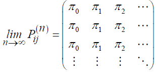
be the row vector such that

We claim that π is a stationary distribution. To show this, consider the equation πP =π . Hence, we have:

Since

, we can substitute π_j into the equation

Next, we show that the stationary distribution is unique. Suppose there exist two stationary distributions

then, we have πP

Consider the difference:

Since both

are probability distributions, the sum of their components is 1:

This implies that

, proving the uniqueness of the stationary distribution of the Markov chain. Hence, the existence of a limiting distribution implies the existence of a unique stationary distribution.

Knowing this, notice how the heat maps indicate a pattern, suggesting the existence of a limiting distribution and, by consequence, the existence of the stationary distribution. These patterns are vital in understanding the stochastic behavior of prime gaps and their probabilistic distribution as shown in Figure 1.

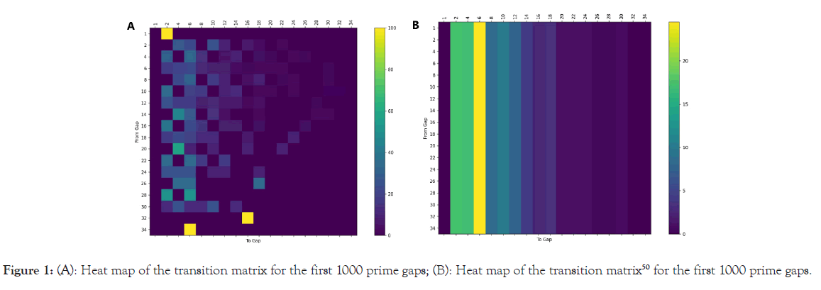
Figure 1: (A): Heat map of the transition matrix for the first 1000 prime gaps; (B): Heat map of the transition matrix⁵⁰ for the first 1000 prime gaps.

Stationary distribution

Lemmas: These are intermediate propositions used to assist in the proof of a larger theorem or statement. They serve as stepping stones, simplifying complex arguments by breaking them down into more manageable parts, thereby enhancing clarity and rigor in mathematical reasoning [7].

Lemma 0: Let

be the sequence of prime gaps. Then,d^_n ≤ 6 infinitely often. (This is also referred to as Tao’s Lemma [8]).

Proof: Suppose, for the sake of contradiction, that Proof: Suppose, for the sake of contradiction, that d_n ≤ 6 for all sufficiently large n. This implies that there exists an integer N such that for all n ≥ N , d^_n ≤ 6 . In other words, there exists a point beyond which every prime gap exceeds 6. Consider the sequence of primes {P_n}. If d_n ≤ 6 for all n ≥ N , this implies that the primes are becoming increasingly sparse as n increases. Specifically, the gaps between consecutive primes are at least 7. However, the prime number theorem tells us that the gaps between consecutive primes P_n are asymptotically approximated by log (P_n). While this allows for large gaps, it does not support the idea that all gaps beyond a certain point are strictly greater than 6. In fact, it is known that there are infinitely many pairs of primes (twinprimes) that are only 2 units apart. This directly contradicts the assumption that d_n ≤ 6 for all sufficiently large n. Thus, our initial assumption must be false, and it follows that there must be infinitely many n for which d_n ≤ 6 .

Lemma 1: Let dn be the most recent prime gap and d_n ≠ d_n−k for k = 1,2,...,(n−1). Then, d_n+k ≤ M where, M = max{d _j}for j=1,2,...,n+1.

Proof: Suppose, for the sake of contradiction, that d_n+1 > M for all n. This implies that dn < d_n+1 for all n, leading to an unbounded sequence of increasing even numbers. This contradicts Tao’s Lemma, which states that gaps less than or equal to 6 occur infinitely often. ⇒⇐ Therefore, our initial assumption must be false, and it follows that d_n+1 > M .

Both lemmas ensure that each new prime gap will connect to previous states.

Irreducibility: A Markov chain

with state space S is said to be irreducible if for any two states i, j ∈ S, there exists a positive integer n such that the n-step transition probability

Formally, this can be expressed as:

Irreducibility implies that it is possible to reach any state from any other state in a finite number of steps.

Theorem 1: Let {X_n} be the Markov chain of prime gaps. Then, all states of {X_n} communicate with each other. Hence, {X_n} is irreducible.

Proof: We need to show that j₁=2 communicates with all other states. Through enumeration, we find that j₁=2 communicates with {4,6}. Consider the one-step transition matrix P=(P_ij). Let {j_k} for k ≥ 4 be the state’s such that

For k=4, j₄=8 and P_4,8=0:,

Thus, m=2. Therefore, it is possible to transition from 2 to 8 in 2 steps. Similarly, since

:

This indicates that transitioning from 8 to 2 is possible via a gap of 4, hence 2↔8. By Lemma 1, 2 communicates with 2k for k ≤ 4. Assuming 2↔2k for all k, we must show that 2↔2 (k+1). By Lemma 1, 2 (k+1) is accessible from at least one smaller prime gap {2k,2 (k − 1),2(k−2)...,2}. Since 2 communicates with all smaller prime gaps, 2 (k+1) is accessible from 2. The prime gap 2k, prior to 2(k+1), communicates with 2, hence 2 is accessible from 2 (k+1). Thus, 2 communicates with 2 (k+1), i.e., 2 ↔ 2 (k+1).

Aperiodicity: A state i ∈ S of a Markov chain is said to be aperiodic if the greatest common divisor (gcd) of the set of return times to i is 1. The chain is aperiodic if all states are aperiodic. Formally, for a state i ∈ S, let:

The state i is aperiodic if d(i)=1. The entire Markov chain is aperiodic if: ∀i ∈ S, d(i)=1

Theorem 2: The states {X_n} are aperiodic.

Proof: Given that P₂₂ ≠ 0 , it follows that d_i=1. Since all states communicate with 2, all states are aperiodic.

Positive recurrence: A state i ∈ S is positively recurrent if the expected return time to i is finite. Let T_i be the first return time to state i. The state i is positively recurrent if:

The Markov chain is positively recurrent if all states are positively recurrent.

Theorem 3: All states of {X_n} are positive recurrent.

Proof: For a fixed number of states S = {j₁, j₂,…, j_m}, Theorem 1 and Theorem 2, show that {X_n} is positive recurrent.

We use induction on the number of states m. Let

and assume the statement is true for k=m. Suppose P_{2, jm+1} = 0 . By Theorem 1, there exists a state jl with 1 ≤ l ≤ m such that P_{2, jl} ≠ 0 and P_{jl, jm+1} ≠ 0 , indicating that j_m+1 communicates with 2. Hence, j_m+1 is positive recurrent.

Ergodicity: A Markov chain is said to be Ergodic if it is irreducible, aperiodic, and positively recurrent.

Theorem 4: The Markov chain of prime gaps is ergodic.

Proof: To establish that the Markov chain {X_n} of prime gaps is ergodic, we need to verify that it satisfies the conditions of irreducibility, aperiodicity, and positive recurrence.

From Theorem 1, we have shown that all states of {X_n} communicate with each other. Hence, the Markov chain is irreducible.

From Theorem 2, it is established that the states {X_n} are aperiodic since P₂₂ ≠ 0 and all states communicate with 2. Thus, the chain is aperiodic.

From Theorem 3, all states of {X_n} are shown to be positively recurrent. Since {X_n} is irreducible, aperiodic, and positively recurrent, it follows that the Markov chain of prime gaps is ergodic. Consequently, the Markov chain {X_n} has a unique stationary distribution

Furthermore, the distribution of states converges to the stationary distribution, i.e.,

Where μ_n is the state distribution at time n and

denotes an appropriate norm such as the total variation norm.

Since the Markov chain of prime gaps is irreducible, aperiodic, and positive recurrent, it is ergodic. Therefore, the Markov chain has a stationary distribution π such that, π P =π

Modular pattern of prime gaps

Visual pattern: In this section, we identify a modular pattern in prime gaps. Specifically, we categorize prime gaps based on their congruence modulo 6 to simplyfy the pattern.

The following categorization reveals a significant structure in the distribution of prime gaps. The histogram illustrates the distribution of prime gaps modulo 6, with each category of bins represented in different colors for clarity. This pattern not only supports our theoretical findings but also highlights the regularity and structure inherent in the distribution of prime numbers as shown in Figure 2.

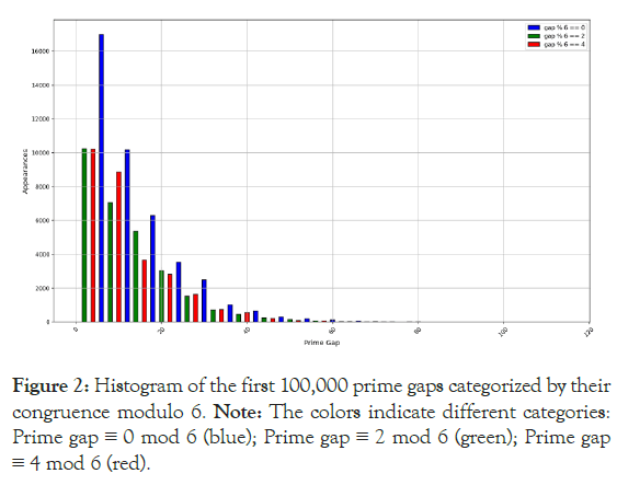
Figure 2:Histogram of the first 100,000 prime gaps categorized by their congruence modulo 6.

Note: The colors indicate different categories: Prime gap ≡ 0 mod 6 (blue); Prime gap ≡ 2 mod 6 (green); Prime gap ≡ 4 mod 6 (red).

Arithmeticity of prime numbers:

Theorem 5: Every prime number p>3 can be written in the form 6k ± 1 for some k ∈ Z.

Proof: Given any integer p>3, we know by the division algorithm that there exist unique integers q ≥ 0 and r ∈ {−1,0,1,2,3,4} such that: p = 6q + r . Suppose that p is prime. Then observe that r≠{0, 2, 4} , since otherwise p would be even (contradicting the fact that p ≠ 2 )⇒⇐. Likewise, observe that r ≠ 3 , since otherwise p = 6q + 3 would be divisible by 3 (contradicting the fact that p ≠ 3 ) ⇒⇐So, r = ±1, as desired.

Prime gaps modulo 6:

Theorem 6: Approximately 50% of prime gaps are congruent to 0 mod 6 and approximately 25% of prime gaps are congruent to 2 mod 6.

Proof: Given that we proved that prime gaps have a stationary distribution, this implies that the probabilities of prime gaps falling into different congruence classes modulo 6 stabilize over time. Therefore, the long-term proportions of prime gaps that are 0 mod 6, 2 mod 6, and 4 mod 6 will remain constant. And since the primes are equally likely to be 6k+1 or 6k-1, and the stationary distribution reflects these equal probabilities, it follows that:

Prime factorization of prime gaps

Prime factorization of even numbers:

Theorem 7: Every prime gaps greater than 1 can be factorized in at least one of the following six ways: 2^a· q, 2^a ·3^b ·q, 2^a ·5^b ·q, 2^a ·7^b ·q, 2^a ·11^b ·q, and 2^a ·3^b ·5^c ·q

Where, a, b, and c are non-negative integers, and q is an odd integer.

Proof: Let

represent the prime gap between two consecutive primes p_n and p_n+1, where, 1 g_n > . According to the Fundamental Theorem of Arithmetic, every integer g_n greater than 1 can be factored into primes.

• Factorization into powers of 2: Any integer can be factored into powers of 2. If g_n is divisible by 2, this is captured by 2a.

• Divisibility by small primes: If g_n is divisible by 3, 5, 7, or 11, it can be captured by the inclusion of 3^b, 5^b, 7^b, or 11^b in the factorization.

• Odd integer q: Any remaining factor that is not divisible by 2, 3, 5, 7, or 11 is captured by q, which must be an odd integer.

Prime factorization pattern in prime gaps

Using Theorem 5 and Theorem 6, we will patternize the prime gaps by determining the percentage of prime gaps that fall into each category based on their prime factorization.

Theorem 8:

• Approximately 19.96% of prime gaps can be factorized as 2^a · q

• Approximately 33.33% of prime gaps can can be factorized as 2^a · 3^b · q

• Approximately 20% of prime gaps can be factorized as 2^a · 5^b · q

• Approximately 14.29% of prime gaps can be factorized as 2^a · 7^b · q

• Approximately 9.09% of prime gaps can be factorized as 2^a · 11^b · q

• Approximately 3.33% of prime gaps can be factorized as 2^a · 3^b · 5^c ·q

Where, a, b, and c are non-negative integers, and q is an odd integer.

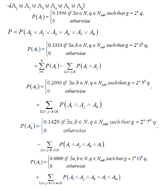
Proof: Prime gaps can be seen as even numbers, so they can be analysed by considering their divisibility by small primes (since every prime gap g>1 is even). The proportion of numbers divisible by 2, 3, 5, 7, and 11 among all even numbers can be approximated using the following reasoning:

Prime gaps divisible by 2a · q where q is not divisible by 3, 5, 7, or 11:

• Prime gaps divisible by 2a · 3b · q where q is not divisible by 5, 7, or 11:

• Prime gaps divisible by 2a · 5b · q where q is not divisible by 3, 7, or 11:

• Prime gaps divisible by 2a · 7b · q where q is not divisible by 3, 5, or 11:

• Prime gaps divisible by 2a · 11b · q where q is not divisible by 3, 5, or 7:

• Prime gaps divisible by 2a · 3b · 5c · q where q is not divisible by 7 or 11:

However, it is important to note that these events are not disjoint, i.e. 60 ≡ 0 (mod 2,6,10,14,22,30). Therefore, the probability of the union of all given states is:

Approximation of expectation

In this section, we approximate the expectation of prime gaps using a sample of 1 billion prime gaps.

By applying logarithmic polynomial fitting to the data, we estimated the formulas for the expectation and variance of a given set of n consecutive prime gaps.

Logarithmic polynomial and fitting: A logarithmic polynomial is a polynomial function in terms of the natural logarithm of a variable. It is generally expressed in the form:

Where, a₀,a₁,...,a_k are coefficients and k is the degree of the polynomial.

Logarithmic polynomial fitting is a statistical method used to approximate a set of data points by finding the coefficients a₀,a₁,...,a_k that best fit the data in a least-squares sense. The goal is to minimize the sum of the squared differences between the observed values and the values predicted by the polynomial model. Formally, given a set of data points (n_i,y_i) for i=1,2,...,m, the fitting process involves solving the following optimization problem:

Where,

Knowing this, for a given sample of n=10¹² prime gaps, we approximate

E(n) ≈1.08556674·In(n) + 0.4495518

This formula indicates a linear relationship between the expectation of prime gaps and the natural logarithm of n, adjusted by a constant term.

Probabilistic mass function of prime gaps

Structure of the PMF of prime gaps: Cramer’s conjecture states that the average gap between consecutive primes near a large number n is approximately In(n) [9]. In other words, the gap between the n^-th prime, pn, and the (n+1)^-th prime, pn+1, is bounded by:

This approximation is also supported by the prime number theorem, which states that the number of primes less than or equal to x is approximately:

Consequently, from these two statements, the density of primes around x is given by:

Hence, the average gap length between consecutive primes near x is then:

However, in this research study, we are not basing our calculations on a number x ∈ R; instead, we are basing our calculations on n ∈ N, representing the set of the first n consecutive prime gaps. Thus, we need to adapt Cramer’s conjecture and the prime number theorem on n: the set of the first n consecutive prime gaps.

Given primes p₁, p₂,…, p_n, the average prime gap length is the total gap divided by n−1, the number of gaps.

Let p_n be the n-th prime. The prime number theorem approximates p_n as p_n ≈ n · ln (n). Plus, the total gap length between the first n primes is approximately 2p_n − , since the first prime is 2. So, for large n, the average gap g_n between the first n primes is then:

This result aligns with Cramer’s conjecture and the Prime Number Theorem, indicating that the average gap between consecutive primes increases logarithmically with the number of primes considered.

Now based on this, we can proceed. Knowing that n represents the number of prime gaps, the simplest model for the gap

is that it follows approximately an exponential distribution of parameter

Following from that, the probability that

is not prime is about:

Best approximation of the PMF of prime gaps

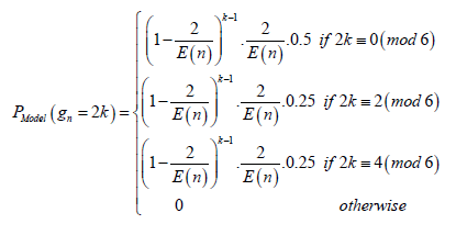
Models to be tested: Based on all of these results, we will analysed compare different models of approximated PMFs for P(g_n=2k) to see which approximation fits better the real PMF of Prime Gaps:

Model 1 and 2:

With:

–Model 1: E (n) ≈ In (n) –Model 2: E (n) ≈1.08556674·In(n) + 0.4495518

Model 3 and 4:

With:

–Model 3: E (n) ≈ In (n) –Model 4: E (n) ≈1.08556674·In (n) + 0.4495518

Model 5 and 6:

With:

–Model 5: E (n)≈ In (n) –Model 6: E (n) ≈1.08556674·In (n) + 0.4495518

Statistical tests

We will compare these 6 different models to determine which best approximates the true Probability Mass Function (PMF) of prime gaps. The following statistical tests will be used on sample sizes of n = 10³, 10⁶, 10⁹, and 10¹² prime gaps to assess the impact of sample size on model performance:

• Chi-Square test: Assesses the difference between observed and expected frequencies:

• Kolmogorov-Smirnov test: Compares the empirical and reference cumulative distribution functions:

• Anderson-Darling (AD) test: Measures how well data fits a specified distribution, improving sensitivity at distribution tails:

With, S representing a modified sum of differences between empirical and theoretical distributions. However, another common form for a finite sample is:

• Mean Squared Error (MSE): Quantifies the average squared difference between observed and predicted values;

• Kullback-Leibler Divergence (KL Divergence): Measures divergence between true and predicted probability distributions;

Notice that Non-parametric statistics, such as the K-S and Anderson- Darling tests, are particularly useful when no specific parametric distribution is assumed, allowing for a more flexible evaluation of model fit. These tests, combined with parametric approaches like the Chi-Square Test, provide a robust framework to evaluate how well the models to empirical data and determine which best approximates the prime gap distribution.

Results

Please note that the graphs below have been adapted up to k=21 to enhance readability and make the results easier to interpret.

Sample Size: n =10³ as shown in Table 1. Sample size: n =10⁶ as shown in Table 2. Sample size: n =10⁹ as shown in Tables 3. Sample size: n =10¹² as shown in Figure 3 and Table 4.

Table 1: Combined test results with best results highlighted, n=10³.

Table 2: Combined test results with best results highlighted, n =10⁶ .

Table 3: Combined test results with best results highlighted, n= 10⁹.

Table 4: Combined test results with best results highlighted, n= 10¹².

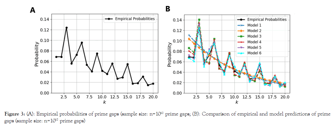
Figure 3:Empirical probabilities of prime gaps (sample size: n=10¹² prime gaps; (B): Comparison of empirical and model predictions of prime gaps (sample size: n=10¹² prime gaps)

Discussion

Test specific observations

The models under consideration can be categorized into three distinct groups based on their approach to the prime gaps:

• Category 1: Basic models (Models 1 and 2)-These models do not incorporate any specific categorization of prime gaps, relying solely on a fundamental approximation of E(n).

• Category 2: Modulo 6 congruence models (Models 3, 4,)-These models classify prime gaps based on their congruence modulo 6, capturing the periodic properties inherent in prime distributions.

• Category 3: Prime factorization models (Models 5 and 6)-These models categorize prime gaps based on their prime factorization, leveraging the deeper arithmetic structure of the gaps.

While all three categories exhibit commendable performance, effectively approximating the PMF of prime gaps to a significant extent, notable distinctions emerge across different statistical tests. For all tests, excluding Anderson-Darling (AD) test, the category 3 models, which incorporate prime factorization, consistently demonstrate the highest accuracy, followed by category 2 models that consider modulo 6 congruence. The basic models in category 1 rank the lowest. This trend underscores the superiority of models that account for more intricate arithmetic structures.

Interestingly, the AD test results deviate from the aforementioned trends. Category 1 models attain the highest ranking in this test. This anomalous result can be attributed to the AD test’s sensitivity to the tails of the distribution. The basic models’ simplicity and broader assumptions may lead to a better fit for the extreme values of the prime gap distribution, explaining their superior performance in this specific test.

Approximation of the expectation of prime gaps: The expectation of prime gaps, E (n) , is an essential parameter in accurately modeling the distribution of gaps between consecutive prime numbers. It is generally approximated by the natural logarithm of n, i.e., E (n) ≈ In (n) . This approximation is widely accepted in number theory due to its basis in the prime number theorem, which states that the average gap between consecutive primes near a large number n is approximately In (n) . However, our analysis shows that more refined approximations of E (n) can significantly improve the accuracy of models, E (n) ≈1.08556674·In (n) + 0.4495518 In summary, while E (n) ≈ In (n) is a widely known and useful approximation, incorporating refined estimates of E (n) can lead to more accurate models of the distribution of prime gaps. These refinements account for empirical observations and theoretical insights that extend beyond the basic logarithmic approximation.

Geometric structure: All the models considered in this study follow a geometric Probability Mass Function (PMF) structure. This choice is based on the assumption that the distribution of prime gaps can be effectively approximated using a geometric distribution. The general form of the geometric PMF used in these models is:

Where, E (n) represents the expected value, which varies across different models. This structure implies that the probability of observing a gap of size 2k between consecutive primes decreases exponentially with k, consistent with the properties of geometric distributions.

The geometric PMF structure captures the idea that larger prime gaps are less likely than smaller ones, a characteristic feature of prime gaps. In other words, the geometric PMF inherently incorporates an exponential decay, reflecting the decreasing likelihood of larger prime gaps, which aligns well with empirical observations.

Piecewise approximations: The comparative analysis reveals that piecewise approximations, which categorize prime gaps based on modulo 6 congruence or their prime factorization, consistently outperform non piecewise approximations. This observation suggests that the PMF of prime gaps exhibits a combinatorial nature influenced by specific sub-properties intrinsic to the prime numbers themselves:

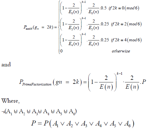
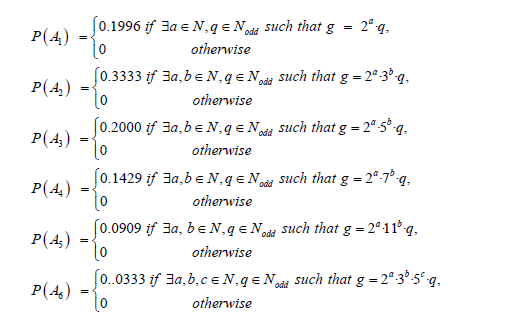
The superior performance of piecewise models highlights the necessity of incorporating de tailed arithmetic properties and combinatorial classifications when approximating the PMF of prime gaps. This approach not only provides a more accurate fit to empirical data but also aligns with the intrinsic mathematical complexities of prime distributions.

Best approximation: The overall best approximation for the PMF of prime gaps is provided by Model 6. This model leverages a sophisticated combinatorial approach, integrating the arithmetic proper ties of prime numbers and utilizing both prime factorization and refined expectation.

• Model 6:

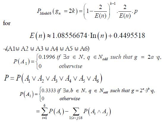
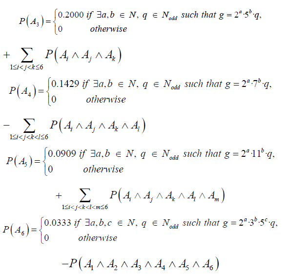
The superior performance of Model 6 implies that the best approximation for the PMF of prime gaps must be a combinatorial PMF that leverages the arithmetic properties of prime numbers. Specifically, it suggests that modular behaviors of the gaps, as well as the prime factorization of even numbers, are important in accurately modeling prime gaps. The intricate structure captured by model 6, which combines these properties, provides a more precise fit for the empirical distribution of prime gaps as shown in Figure 4.

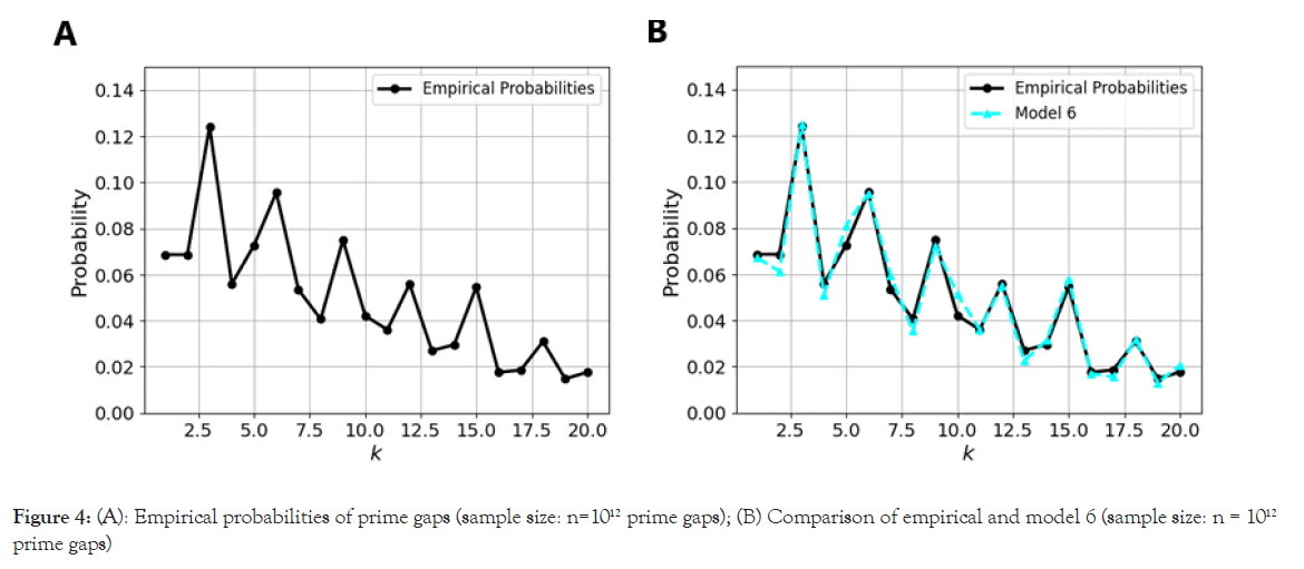
Figure 4: (A): Empirical probabilities of prime gaps (sample size: n=10¹² prime gaps); (B) Comparison of empirical and model 6 (sample size: n = 10¹² prime gaps)

Moreover, the combinatorial nature of this approximation can also influence E(n) , indicating that the formula for the average gap length must be more complex than just E (n) ≈ In (n) . The refined function

E (n) ≈1.08556674·In (n) + 0.4495518 used in model 6 underscores this complexity, suggesting that a more sophisticated understanding of prime gaps involves a detailed analysis of their arithmetic properties and combinatorial classifications.

Results-based conjecture

Hypotheses: Based on the empirical results obtained and the comprehensive investigation conducted, we hypothesize that the Probability Mass Function (PMF) of prime gaps exhibits a uniform distribution for gaps of size 2 and 4, while for larger gaps, it follows a more complex structure. Specifically, we conjecture that the PMF of prime gaps from 6 onward is best described by an infinite combination of geometric distributions, each corresponding to a distinct prime factorization of even numbers. This framework suggests a deep connection between the arithmetic properties of integers and the distribution of prime gaps, providing a novel perspective on their underlying structure.

Conjectures:

Conjecture 0: The percentage of prime gaps of length 2 and length 4 among all prime gaps is approximately 5% for both gaps respectively. I.e. for π being the stationary distribution of prime gaps, then π₂ = π₄ ≈ 0.05.

Proof: First we will prove that as n approaches infinity, the percentage of prime gaps of lengths 2 and 4 asymptotically converges to the same value. We’ll combine the provided model for prime gaps, the given probabilities P(A_i), and theorems related to the distribution of prime gaps.

Theorem 4, indicates that the Markov chain made of prime gaps has a stationary distribution, implying that the proportion of different prime gaps stabilizes as n increases. And based on the outstanding performance of model 6 in approximating the probabilistic distribution of prime gaps, we will use it to compute the probabilities of specific

prime gaps:

• Model 6:

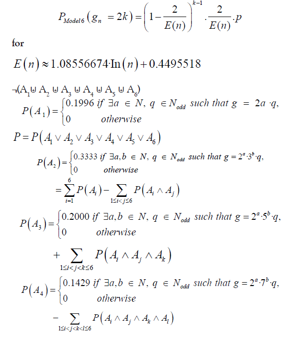
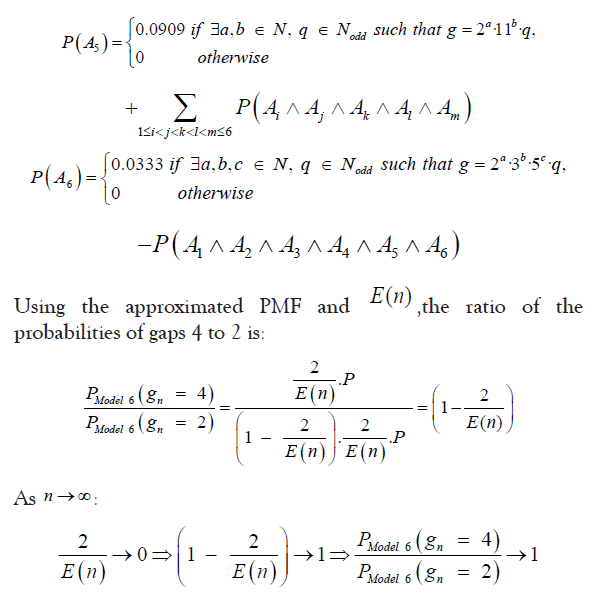
Given the existence of a stationary distribution of the Markov chain made of prime gaps, the probabilities for gaps of lengths 2 and 4 converge to the same asymptotic value. Let the prime counting function π be our stationary distribution:

The twin prime conjecture states that there are infinitely many pairs of primes ( p, p + 2) where the gap between the primes is 2. Although this conjecture has not yet been proven, substantial evidence supports its validity.

Empirically, it is observed that prime gaps of length 2 are quite frequent among smaller primes. However, as numbers get larger, the distribution of prime gaps becomes more varied. Despite this, twin primes continue to appear even among large numbers, though less frequently.

Let π₂ (x)be the number of twin primes less than or equal to x, and π (x) be the total number of primes less than or equal to x . The proportion of twin primes relative to all primes can be estimated using:

Where, C₂ is the twin prime constant, approximately 0.660161. Using the prime number theorem:

While an exact percentage is difficult to calculate without exhaustive data, we can use empirical and asymptotic results to estimate the percentage of prime gaps that are length 2.

According to these estimates, the proportion of twin primes (gaps of 2) tends to:

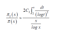
For practical purposes, over large ranges of x, this ratio typically falls in the range of 5%-6%. Empirical studies and computational data on prime numbers suggest that the percentage of prime gaps that are exactly 2 among all prime gaps is approximately 5% for large ranges of primes. After having proved that states that he percentage of prime gaps of lengths 2 and 4 asymptotically converges to the same value, we conclude:

Percentage of prime gaps of length 2=Percentage of prime gaps of length 4 ≈ 5% to 6%

Conjecture 1: The Probability Mass Function (PMF) of prime gaps for gaps of size 6 and greater follows an infinite combination of geometric distributions determined by the prime factorization of even numbers. More precisely, the Probability Mass Function (PMF) of prime gaps is uniform for gaps of size 2 and 4, and for gaps of size 6 and greater, it follows an infinite combination of geometric distributions determined by the prime factorization of even numbers.

Based on our results, hypothesize that the distribution of prime gaps, denoted by the Probability Mass Function (PMF) P(g_n), can be expressed as an infinite sum of weighted geometric distributions. Each geometric distribution corresponds to a specific category, defined by the prime factorization of the even number representing the prime gap. The more categories we include in our model, the more precise our approximation of the prime gap distribution becomes. In the limit, as the number of categories approaches infinity, the model converges to the exact distribution of prime gaps.

Let C represent the set of all possible prime factorizations of even numbers, and let Ci denote a specific factorization category. Then, the PMF (g_n=2k) can be expressed as:

•P_i(g_n=2k) is the geometric PMF for the i-th factorization category Ci.

• W_i is the weight assigned to the i-th category, representing the proportion of prime gaps that fall into this category.

• The sum extends over all possible categories Ci, corresponding to all possible prime factorizations of even numbers.

As the number of categories in C increases, the sum becomes more inclusive of the different possible factorizations of prime gaps. In the limit, as the number of categories approaches infinity, the model becomes fully precise, capturing the exact distribution of prime gaps:

This model suggests that prime gaps are deeply connected to the arithmetic structure of integers. Their distribution can be understood as a complex, yet structured, combination of simpler geometric distributions. The more we account for the different prime factorizations, the more accurately we model the true distribution of prime gaps.

Thus, we conjecture:

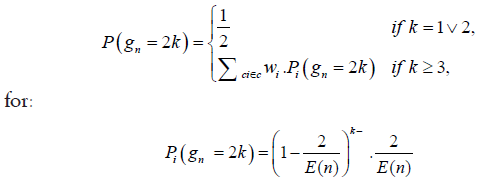
Where E (n) is the expectation of the prime gaps, and W_i is the weight associated with the i-th prime factorization category C_i.

Conclusion

This study has provided significant insights into the distribution of prime gaps, emphasizing the importance of models that incorporate arithmetic and combinatorial properties. We categorized models into three groups: Basic, modulo 6 congruence, and prime factorization models. Among these, prime factorization models consistently yielded the most accurate predictions, particularly for larger prime gaps, high lighting the intricate arithmetic structures that influence prime gaps.

A critical advancement in this research is the refinement of the expectation of prime gaps, E (n) . The refined function, E (n) ≈1.08556674·In (n) + 0.4495518, offers a more precise estimate than the traditional logarithmic approximation, improving model accuracy, especially when combined with a piece wise approach.

The geometric Probability Mass Function (PMF) structure effectively captures the exponential decay of prime gaps, with larger gaps becoming increasingly rare. This study led to conjecture 1, which posits that while the PMF of prime gaps is uniform for gaps of size 2 and 4, it follows an infinite combination of geometric distributions for gaps of size 6 and greater, determined by prime factorization. This conjecture highlights the dual nature of prime gaps-simple and uniform for small gaps, but complex and structured for larger ones.

Prime factorization serves as a critical factor in understanding these larger gaps, suggesting that the distribution of prime gaps is not random but deeply connected to the arithmetic properties of integers. The more complex the factorization, the more intricate the gap’s distribution becomes. In conclusion, conjecture 1 offers a unifying framework that links small, uniform gaps with larger, more complex gaps through the lens of prime factorization. Future research should focus on testing and refining this conjecture, potentially uncovering deeper connections between prime numbers and their gaps.

References

1. Euclid, Elements. Clark Univers. 1996.
2. Hardy GH, Littlewood JE. Some problems of ‘Partitio numerorum’; III: On the expression of a number as a sum of primes. Acta Math. 1923;44(1):1-70.

   [Crossref] [Google Scholar]

3. Erdos P. On the difference of consecutive primes. Q J Math. 1935;6(1):124-128.

   [Crossref] [Google Scholar]

4. Goldston DA, Motohashi Y, Pintz J, Yıldırım CY. Small gaps between primes exist. Proc Japan Acad Ser. A Math. Sci. 82(4): 61-65

   [Crossref] [Google Scholar]

5. Zhang Y. Bounded gaps between primes. Ann Math. 2014;179:1121-1174.

   [Crossref] [Google Scholar]

6. Hadamard J.  On the distribution of zeros of the function and its arithmetic consequences. Bull Soc Math Fr. 1896; 24:199-220.

   [Crossref] [Google Scholar]

7. Abdullah D, Rahim R, Apdilah D, Efendi S, Tulus T, Suwilo S. Prime numbers comparison using sieve of eratosthenes and sieve of sundaram algorithm.  J Phys Conf Ser. 2018;978:012123.

   [Crossref] [Google Scholar]

8. Tao T. Every odd number greater than 1 is the sum of at most five primes. Math Comp. 2014;83(286):997-1038.

   [Crossref] [Google Scholar]

9. Cramér H. On the order of magnitude of the difference between consecutive prime numbers. Acta Arith. 1936;2: 23-46.

   [Crossref] [Google Scholar]