Journal of Proteomics & Bioinformatics
Open Access
ISSN: 0974-276X
ISSN: 0974-276X
Research Article - (2024)Volume 17, Issue 3
In the aim of presenting a learning approach derived from algebraic topology for protein structure prediction, we will be showing how our quotient spaces could qualitatively give insight into how building good homomorphism’s can help identifying accurate neural networks. We will also be giving as an example of application the use of a model generated after extracting an algebraic invariant which is in our case a persistent diagram on some biological data, by encoding the two first homologies H1 to H0 using a boundary operator, the algorithms are originated from algebraic geometry. Basically two main algorithms are used the Buchberger’s algorithm and Shreyer’s algorithm.
Neural networks; Persistent diagrams; Buchberger’s algorithm; Shreyer’s algorithm
The main idea of this paper is reconstructing molecular shapes by using alternative to the interpreted graph neural networks that are using geometric parametres for building artificial intelligence models, so we can access a theoretical justification of the topological signature from our previous work and explore new topological models for application purposes [1]. We will be considering the metrical representation of a boundary operator defined on the set of edges to the set of vertices in the context of an affine varieties so we can reconstruct the variety from an already defined algebraic topological space, let’s illustrate by a first example, the following is a filtered simplicial table.
A quantification of the boundary operator obtained from Grobner and Buchberger algorithms using ideals as basis generators to solve a hidden polynomial equations system would be;
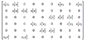
The two following theorems will play a central role in road mapping the inverse of the boundary and would also give us a justification to work in a commutative algebraic setting.
Theorem 1. (Strong Nullstellensatz) If K is an algebraically closed field and I is an ideal in K[x1, ..., xn] then
I (V (I )) = √ I
Theorem 2. (Ideal-Variety Correspondence) Let K be an arbitrary field; the maps
Affinevarieties→ideals
and
ideals→ Affinevarieties
are inclusion reversing and
V (I (V )) = V
for all affine varieties V, if K is an algebraically closed then
Affinevarieties→radicalideals
and
radicalideals→ Affinevarieties
are inclusion reversing bijections and inverses for each other. Our free resolution is guaranteed from the following theorem. Theorem 3. The boundary of a boundary vanishes, that is;

Proof. We have;

Then


= 0
Let’s now detail the computing part of the previous.
Persistent diagram with different methods of construction
Let’s consider the following revision from which we can derive a clear description of the class of linear statistical representations;
X × Y
as universal components in a set theoretical context.

It is now sufficient to consider the pushout of the precedent diagram so the existence of our persistent diagram is guaranteed. Let us now involve more components to full-fill the definition, for that reason and to exploit efficiently theorems and proofs of the investigated theory, let us consider the functoriality of the main definition,

With ψ ,ϕ are well defined vertex mappings between different set vertices contained in a filtered simplicial complexes, we should also mention that no theoretical frame or applied one is given in the literature for a comparison between kernel density estimation construction vs alpha complex one of the persistent diagram in topological data analysis.
To be able to visualize the filtration process, one needs to consider the pullback given by,
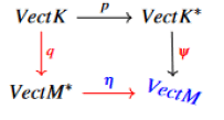
Then given a sequence of inclusions of topological spaces

and its homology groups cautioned by their tames, a persistent diagram up to isomorphism is given by the following;
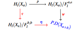
The inclusions of topological spaces induces immediately an inclusion between the cautioned spaces, we now can be sure from the greatest lower bound which is

This gives a theoretical frame to construct our confidence sets intervals. We should mention before getting in the proposed probabilistic models or the way they are writing that computer simulations nowadays made the theoretical frame quite flexible but less deliberate, especially when a new theory is proposed. This is the case with persistent diagrams. We should also mention that persistent diagrams are either derived from a learning process or functional summaries within a larger Hilbert space, for that reason one should investigate how the replicated persistent diagrams can be generated and what makes it different from other traditional constructions, principal component analysis as an example. To prove existence and definition of a replicated persistent diagram, we will be solving the problem of replication by investigating the behaviour of a persistent diagram near its greatest lower bound given by following [2].

From the already defined inclusion of topological spaces, we derive the following commutative diagram;

then we induce by using relative homology the following exact sequence;

Which means the caution could be defined for the whole inclusion, then a replicated persistent diagram is theoretically guaranteed. To fulfill the definition we consider the following diagram.

The uniqueness of our persistent diagram to conclude the definition depends on a factorization of the previous in the functor h back to the previous relative sequence we have.
p, q ∈ H* are well defined projections which implies H ∈ W it is now sufficient to prove Imp ∈ W or Imp ∈ Hl or (Xa)/Fl b,b ∈ H* the second inclusion is given by construction or in Hl(Xa)/Fl b,b every map calculate a homology within Fl b,b we confirm that W has the same topological degree as P.D(Xa+b) which gives the commutativity of the diagram. We conclude the uniqueness of P.D(Xa+b) then P.D(X) for any topological space (X) with some degree p.
Being said, the immediate way to start is building a confidence set interval for 
With  is an estimate of the persistent diagram constructed from a sample.
W∞ is the bottleneck distance, we consider for that reason the theorem.
Theorem 4. Let f, g : K → R be monotone functions. Then;

for a homology dimension k we have;

We then bound
H ( S, M )
such that H is the Hausdorff distance;

to obtain a bound on

with ε = Z(VectM*)
We can now easily define a 1 − α confidence set interval for the bottleneck distance;

that is;

With pn an adequate statistical descriptor of  the last step is to find α such that

Then the set of persistent diagrams are given.
 such that; Cn is the confidence set related to
  .
.
Being said, we get a confirmed theoretical frame to start the statistical study that involve point clouds representing atoms lying in a high dimensional space with a hidden locally Euclidean manifold. The next step consists of presenting algorithms derived from the previous result mentioned in the introduction, which is persistent homology of filtered complex is nothing but the regular homology of a graded module over a polynomial ring [3-6].
Polynomial solutions of boundary operators
Boundary and cycles modules: The concept of boundary and cycles is theoretically formalized in the previous definition of a persistence homology, homology gives a description of the set of cycles, by using the caution over the set of boundaries, which also means by persistence, preserving the cycles that are not boundaries.

In our context, cycles are the significant topological signatures of all types including loops and loops of loops, holes and cavities and so on. Let’s now compute our homologies, as already mentioned in the introduction persistent homology of filtered complex is nothing but the regular homology of a graded module over a polynomial ring, our module is defined over the n graded polynomial ring;

with standard grading

then
R = An
Then our vector of polynomials is writing as [a1, ..., am]T , ai is a polynomial where the matrix Mi+1 for ∂i+1 has mi rows and mi+1 columns where mj stands for the number of j − simplices in the complex, ai is the ith column in Mi+1 thus we can separate polynomials from the derived coefficients, let

Where aiis the ith column in Mi+1 one now can write a polynomial vector a in a submodule in term of some basis A as in

to get a final result computing ∂i+1. Things seems easier for the cycle submodule, which is a submodule of the polynomial module. As previously, this time ∂i has mi−1 rows and mi columns,

Where ai is the ith column in the matrix, the set of all [q1, ..., qmi]T such that
 is a R submodule of
  which is the first Syzygy module of (a1, ..., ami). A set of generators of the previous would finish the task, then finally to compute our homologies it suffices to verify whether the generators of the Syzygy submodule are in the boundary submodule.
Solving the problem of the boundary within a variety would consists of solving all edges and vertices within a set of polynomials equations without losing topological significance. The inverse inclusion would give an exact sequence for the boundary operators. The problem then takes the form of a free resolution, so we have the following computation.
Computation of homologies and rank invariant: Let’s consider the polynomial module Rm with the standard basis e1, ..., em where ei is the standard basis vector with constant polynomial 0 in all positions except 1 in position i, min Rm is of the form xuei for some i and we say m contains ei. For, u, v ∈ Nn u > v, if u − v ∈ Zn the left most nonzero entry is positive, this gives a total order on Nnas an example (1, 4, 0)>(1, 3, 1) since (1, 4, 0)−(1, 3, 1)=(0, 1, 0) the left most nonzero is 1, for two monomials xu, xv in R, xu>xv if u>v which gives a monomial order on R we then extend the order on Rm by using xuei>xvej if i<j or if i=j and xu>xv, r ∈ Rm can be written in a unique way, as a k linear combination of monomials mi;

Where ci ∈ K, ci ≠ 0 and mi ordered according to monomial order. As an example, if we consider

Then we can write f in terms of the standard basis

We then extend operations such as least common multiple to monomials in R and Rm we summarize them by saying
m / n = xu / xv = xu−v
After a division, we get

So, if r=0 then a ∈ <A> so the division is not a sufficient condition, for that reason we use Grobner basis then by forcing the leading terms to be equal we get a sufficient condition. For unicity and minimality, we reduce each polynomial in G by replacing g ∈ G by the remainder of g/(G − g) then im∂i+1 is well computed.
Still to compute generators for the Syzygy submodule, we compute a Grobner basis.
A = {a1,...,as}
For <A> where the ordering is the monomial one, we then follow the same process as for im∂i+1 we get

with gk elements of the Grobner we need now a Grobner basis for
SYZ (a1,...,as)
which can be obtained by using Schreyer’s theorem, guaranteeing the existence of

otherwise, we use this basis to find generators
SYZ (g1,...,gs)
for a metrical representation we consider elements ai and gi from S as columns of a given MA and MG respectively, the two basis generate the same module. ∃A, B such that MG=MAA, MA=MGB with each column of MA is divided by MG since MG a Grobner basis for MA. We conclude, there is a column in B for each column ai ∈ MA that can be obtained by division of ai by MG. Let;
S1,...,St
be the columns of the t × t matrix It – AB. Then;
SYZ (a1,...,at) =< ASi j, S1,...,St >
Then the Ker∂i is computed. Finally we need to compute the caution Hi given im∂i+1=<G> and Ker∂i=SYZ(a1, ..., at). We divide every column in Ker∂i by im∂i+1 using the same process as in computing im∂i+1 if the remainder is non zero we add it both to im∂i+1 and Hi. Therefore, we count only unique cycles. We obtain for the previous bifiltration the following homogenous matrix for ∂1 So M11 is obtained by cautioning

and so on, the full matrix then has the form
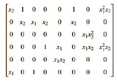
To compute the rank invariant, we can use the multigraded approach, then if we take the previous bifiltration, matrices for SYZ(G1) and Grobner of Z1 for ∂1 are obtained as previously,
Multi-filtered dataset: In topological data analysis, a multifiltered data set can be defined as;
Definition 1. (S, {fj} j), where S is a finite set of d-dimensional points with n – 1 real-valued functions.
fj : S → R
Defined on it, for n>1. We assume our data is a multifiltered dataset (S, {fj} j).
In the following definitions, the calculations are made in commutative algebraic setting, this induces an order on the multifiltration, which can be viewed as an action of a ring over a module plus an inclusion maps relating copies of vertices within complexes, we will be using the ring of polynomials to relate the chain groups in the different grades of the module as the following;

with

For that purpose, let us detail the definition.
Definition 2. A p-dimensional simplex or p − simplex σp = [e0, e1, ..., ep] is the smallest convex set in a Euclidean space Rm containing the p+1 points e0, ..., ep;

Another interesting and explicit description of persistent homology via visualization of barcodes can be found in [7]. We suggest here a concise precise definition via classification theorem.
Remark 1 (Persistence modules). We apply the “homology functor” to the filtered chain complexes, so we get our “homology groups” category [8,9]. This can be viewed as;

Where → denotes the inclusion map.
For a finite persistence module C with filed F coefficients

that are the quantification of the filtration parameter over a field, with clear description [10].
Definition 3. The p-persistence k-th homology group

well defined since Bkl+P and Zlk are subgroups of Ckl+P.
Let us consider the previous bi filtration from the introduction; we assume the computation are in
Z ⊕Z
and u1=(0, 2), u2=(0, 1), u3=(0, 0), u4=(1, 2), u5=(1, 1), u6=(1, 0), u7=(2, 2), u8=(2, 1), u9=(2, 0), u10=(3, 2), u11=(3, 1), u12=(3, 0) to be read from top to the bottom.
In this example, we have F4 in grade (0, 0),
F5=x1 × F4 in grade (0, 0).
F6=x2 × F5= x1 × x2 × F4 in grade (1, 1) and so on, then ∂1 as from

can be computed

Computation of homologies and rank invariant for atoms point cloud: Being said gives a clear road map to start hypothesizing over a real data set. For that reason, let us consider a folding protein that constitutes N particles and has the spatiotemporal complexity of . We assume that our system can be described as a set of N nonlinear oscillators of dimension RnN* R+, where n is the dimensionality of a single nonlinear oscillator. We will be using data from the freely data bank of Protein Data Bank (PDBs), the molecule in consideration has 1cos as an ID. Our point cloud lying in a R3.700, coordinates of atoms are considered as the input of our multidimensional filtration (Figure 1).
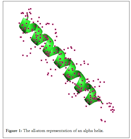
Figure 1: The all-atom representation of an alpha helix.
We obtain in a first sight the following topological signatures which means our final result is a three dimensional simplex (Figure 2).
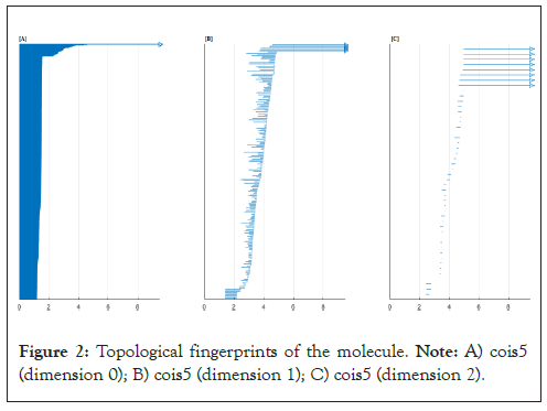
Figure 2: Topological fingerprints of the molecule. Note: A) cois5 (dimension 0); B) cois5 (dimension 1); C) cois5 (dimension 2).
To simplify the task let us consider the alpha carbon atoms of our molecule (Figure 3).
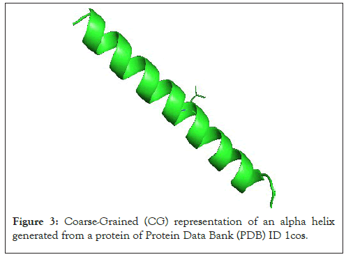
Figure 3: Coarse-Grained (CG) representation of an alpha helix generated from a protein of Protein Data Bank (PDB) ID 1cos.
The topological signature was given in Figure 4.
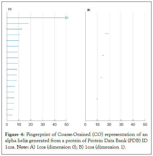
Figure 4: Fingerprint of Coarse-Grained (CG) representation of an alpha helix generated from a protein of Protein Data Bank (PDB) ID 1cos. Note: A) 1cos (dimension 0); B) 1cos (dimension 1).
This means our final result when the end of the multifiltration is a one dimensional simplex, with eighteen vertex at the beginning of the multifiltration; u1=(3, 20, 21), u2=(3, 19, 21), u3=(4, 21, 22), u4=(3, 21, 23), u5=(3, 19, 23), u6=(3, 20, 24), u7=(4, 21, 23), u8=(3, 22, 25), u9=(4, 20, 22), u10=(3, 21, 24), u11=(3, 22, 26), u12=(3, 23, 26), u13=(4, 25, 26), u14 =(4, 24, 25), u15=(4, 19, 25), u16=(3, 23, 19), u17=(4, 23, 26), u18=(4, 22, 27).
We get after calculations the following matrix;
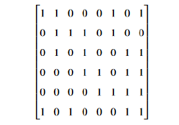
which means the final shape conserve only one type of homology, with four loops as generators. Let us now involve more parameters, we consider decreasing radial basis functions. The general form is;

Where, ωij is associated with atomic types, then a generalized exponential kernel has the form;

k>0 one then can construct the following matrix.

This matrix can easily be obtained following the division algorithm mentioned in the previous section. By considering, xyz coordinates of atoms as the input of the multifiltration, and then the result can be used as the input for the persistent homology calculations following the same process. This clearly shows the path for an easiest extraction of a shape of a protein, since the traditional methods use many complicated parameters to build matrices supposed to rebuild the geometric conformation as the case of molecular nonlinear dynamics and flexibility rigidity index involving exponential kernels with parameters. For more enlightenment through an interesting detailed investigation of topology function relationship paradigm of proteins [3,11].
As we have already mentioned in the previous section a full description of persistent homology can be obtained following; persistent homology of filtered complex is nothing but the regular homology of a graded module over a polynomial ring. The computation is also easy following; a division algorithm then a Buchberger algorithm to seek generators then basis (ideals) for modules. The final step for a statistical analysis is a quantification of the result of the second section to figure out the so-called replicated persistent diagrams. We can observe the significant topological difference between tertiary structures and secondary structures from Figure 5; the interesting task would be a separation between the alpha helices and beta sheets. Those can be literally expressed as the length of the coefficients lying in the metrical representation of our computed quotient Hi [2,12].
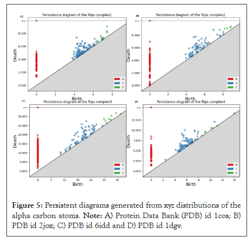
Figure 5: Persistent diagrams generated from xyz distributions of the alpha carbon atoms. Note: A) Protein Data Bank (PDB) id 1cos; B) PDB id 2jox; C) PDB id 6idd and D) PDB id 1dgv.
The total loss function incorporating homology into the learning process is given by;

Where
• L (θ) is the total loss function of the model.
• Loss (f (xi; θ), yi) is the standard loss function for the ith data point.
• f (xi; θ) is the model’s prediction for input xi with parameters θ .
• yi is the true label for the ith data point.
• hj is the homology coefficient for the jth feature or level.
• λ is the regularization parameter that controls the weight of the homology term.
After running the model through our dataset, we get a folding process describing the behavior of different types of homologies through variation of our Gaussian probability distribution.
For a neural network with a single hidden layer, the learning function can be summarized as follows;

Where,
• σ (z) is the activation function (e.g., sigmoid for binary classification, soft-max for multi-class classification).
• L(y, ypred) is the loss function (e.g., binary cross-entropy or categorical cross-entropy).
The parameter updates using gradient descent are given by;


Where,
• η is the learning rate.
• are the gradients of the loss with respect to weights and biases.
Statistical summary of models is given (Table 1, Figures 5-7).
| Metric | DeepCNF (2018) | DNN-Pred (2019) |
|---|---|---|
| Accuracy | ~ 80% | 75%-78% |
| Precision | High for residue-level prediction | Good for domain classification |
| Recall | High for secondary structure tasks | Good for protein interactions |
| Complexity | High (CNN+CRF) | Moderate (MLP) |
| Training data | Large PDB datasets | CASP and other benchmarks |
| Computational cost | High due to CRFs and CNNs | Moderate due to MLP |
Note: DeepCNF: Deep Convolutional Neural Fields; DNN-Pred: Deep Neural Network-based Prediction; CNN: Convolutional Neural Network; CRF: Conditional Random Field; MLP: Multilayer Perceptron; PDB: Protein Data Bank; CASP: Critical Assessment of Structure Prediction.
Table 1: Comparison of DeepCNF and DNN-Pred models.
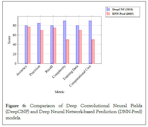
Figure 6: Comparison of Deep Convolutional Neural Fields (DeepCNF) and Deep Neural Network-based Prediction (DNN-Pred) models.
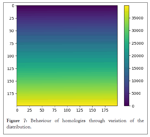
Figure 7: Behaviour of homologies through variation of the distribution.
Experimental procedures
In the all-atom model, atoms are considered the same; each atom is associated with the same radius in the distance-based filtration. The stream will be constructed for the point cloud data, which is the xyz, coordinates of the all atom representation (Figure 8). The size is not too large to choose a landmark selector, so we will simply build a Vietoris-Rips stream. We can choose a better filtration but for the limited computation power, we stick with the value of 8. In this case a Vietoris-Rips complex is largely sufficient to decipher the topological fingerprints (a small data set) so there is no need to use a landmark selector, which can be seen in the code shown below [13-16].
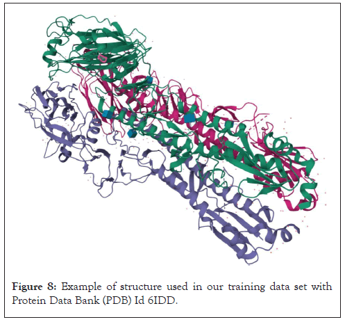
Figure 8: Example of structure used in our training data set with Protein Data Bank (PDB) Id 6IDD.
>> s i z e (ecos)
ans = 696 3
>> max_dimension = 3;
>> max_filtration_value = 8;
>> num_divisions = 1000;
>> stream = api.Plex4.create Vietoris-Rips Stream (ecos, max_dimension , . . . max_filtration_v a l u e, n u m _d i v i s i o n s);
>> n u m _s i m p l i c e s = s t r e a m . g e t S i z e () n u m s i m p l i c e s =3259289
>> p e r s i s t e n c e = a p i . P l e x 4 . g e t M o d u l a r S i m p l i c i a l A l g o r i t h m (max_dimension, 2);
>> o p t i o n s . f i l e n a m e = ’ c o i s ’ ;
>> o p t i o n s . m a x f i l t r a t i o n v a l u e
= m a x f i l t r a t i o n v a l u e ;
>> o p t i o n max_dimension=max_dimension–1;
>> o p t i o n s . s i d e_ b y_ s i d e = t r u e ;
>> p l o t _b a r c o d e s (i n t e r v a l s , o p t i o n s) ;
We utilize the Coarse-Grained (CG) with each amino acid represented by its Alpha Carbon (Cα) atom. The simplices are constructed which is helpful for the detection of the helix structure, so the corresponding barcode is simplified. As the last construction a Vietoris-Rips stream is largely sufficient to decipher the topological features of our data which is an 18 points in a 3-dimensional space. A part of the Matlab© code is shown below.
>> load ecos 1
>> s i z e (e c o s) ans = 18 3
>> m a x_d i m e n s i o n = 2 ;
>> m a x _f i l t r a t i o n _v a l u e =2 3 ;
>> n u m _d i v i s i o n s =1000 ;
>> s t r e a m = a p i . P l e x 4 . c r e a t e V i e t o r i s R i p s S t r e a m (ecos, m a x_d i m e n s i o n, . . . m a x _f i l t r a t i o n _v a l u e , n u m d i v i s i o n s) ;
>> o p t i o n s . f i l e n a m e = ’ c o i i s 2 ’ ;
>> o p t i o n s . m a x f i l t r a t i o n v a l u e = m a x f i l t r a t i o n v a l u e ;
>> o p t i o n s.max dimension=max dimension−1;
>> p e r s i s t e n c e = a p i . P l e x 4 . g e t M o d u l a r S i m p l i c i a l A l g o r i t h m (max_dimension, 2) ;
>> o p t i o n s . s i d e b y s i d e = t r u e ;
>> i n t e r v a l s = p e r s i s t e n c e . c o m p u t e I n t e r v a l s (s t r e a m) ;
>> p l o t b a r c o d e s (i n t e r v a l s , o p t i o n s) ;
for the beta sheet construction, we use the following:
>> l o a d f i n b e t a
>> max_dimension=2;
>> m a x _f i l t r a t i o n _v a l u e = 5 ;
>> n u m _d i v i s i o n s =1000 n u m d i v i s i o n s = 1000
>> s t r e a m = a p i . Plex 4 . c r e a t e V i e t o r i s R i p s S t r e a m (b e t i 0 0 1, max_dimension, . . . m a x _f i l t r a t i o n _v a l u e, n u m _d i v i s i o n s) ;
>> n u m s i m p l i c e s = s t r e a m . g e t S i z e () n u m s i m p l i c e s = 149776
>> p e r s i s t e n c e = a p i . P l e x 4 . g e t M o d u l a r S i m p l i c i a l A l g o r i t h m (max_dimension, 2);
>> i n t e r v a l s = p e r s i s t e n c e . c o m p u t e I n t e r v a l s (s t r e a m) ;
>> o p t i o n s. f i l e n a m e = ’1 bet ’ ;
>> o p t i o n s. m a x f i l t r a t i o n v a l u e = m a x _f i l t r a t i o n _v a l u e ;
>> o p t i o n s.max_dimension=max_dimension–1;
>> o p t i o n s . s i d e b y s i d e = t r u e ;
>> p l o t b a r c o d e s (i n t e r v a l s , o p t i o n s) ;
Then we simplify without loosing topological significance by using the following:
>> l o a d b e t y
>> s i z e (b e t i 0 1) a n s =
24 3
>>max_dimension=2;
>> m a x _f i l t r a t i o n _v a l u e = 2 0 ;
>> n u m d i v i s i o n s =1 0 0 0 n u m d i v i s i o n s = 1000
>> s t r e a m = a p i . P l e x 4 . c r e a t e V i e t o r i s R i p s S t r e a m (b e t i 0 1 , max_dimension, . . . m a x _f i l t r a t i o n _v a l u e , n u m _d i v i s i o n s) ;
>> n u m s i m p l i c e s = s t r e a m . g e t S i z e () n u m s i m p l i c e s = 410
>> p e r s i s t e n c e = a p i . P l e x 4 . g e t M o d u l a r S i m p l i c i a l A l g o r i t h m (max_dimension, 2);
>> i n t e r v a l s = p e r s i s t e n c e . c o m p u t e I n t e r v a l s (s t r e a m) ;
>> o p t i o n s . f i l e n a m e = ’ b e t ’ ;
>> o p t i o n s . m a x f i l t r a t i o n v a l u e = m a x _f i l t r a t i o n _v a l u e ;
>> options.max_dimension=max_dimension−1;
>> o p t i o n s . s i d e _b y _s i d e = t r u e ;
>> plotbarcodes (intervals, o p t i o n s) ;
# −*− coding: utf−8−*−
””” U n t i t l e d 1 . i p y n b ”””
import numpy as np
import m a t p l o t l i b . p y p l o t as plt
import numpy as np
impo
rt seaborn as sns
from matplotlib import colors
from mpltoolkits.mplot3d import Axes3D
import matplotlib.pyplot as plt
from pylab import*
from array import array
pip install pdbreader
import p d b r e a d e r
p d b = p d b r e a d e r . r e a d p d b (” / c o n t e n t / 2 j o x . p d b ”)
from google.colab import drive
d r i v e . m o u n t (’ / c o n t e n t / d r i v e ’)
”””# Nouvelle section ”””
for key in pdb:
print (key)
ATOM = pdb [’ATOM’]
type (ATOM)
for key in ATOM:
print (key)
matrix = [ATOM [’x’]],
ATOM [’y’],
ATOM [’z’]]
p r i n t (m a t r i x)
table=np.empty ((696, 3))
p r i n t (t a b l e)
for i in range (0,696):
table [i] = [np.array (row [i]) for row in matrix]
print (table [i])
a = n p . a s a r r a y (t a b l e)
np.savetxt (”/content/matrixNOTordered.csv”, a, delimiter=”,”)
tabEX = table
print (tabEX)
a = n p . a s a r r a y (t a b E X)
n p . s a v e t x t (” / c o n t e n t / c c . c s v ” , a , d e l i m i t e r =” , ”)
d e f a r r a n g e (t a b E X , n , m) :
for i in range (0, m):
line = tabEX [i] − tabEX [i+1]
for j in range (0, n):
if line [j]<0:
temp = tabEX [i]
tabEX [i] = tabEX [i+1]
tabEX [i+1] = temp
break
elif line [j]>0:
break
elif i<18: print (tabEX [i])
else: continue
return tabEX
print (tabEX)
a = n p . a s a r r a y (t a b E X)
n p . s a v e t x t (” / c o n t e n t / k k . c s v ” , a , d e l i m i t e r =” , ”)
from typing import KeysView
table au = np.empty ((696,3))
for i in range (696, 3):
for j in range (696, 3):
for k in range (0, 2):
t a b l e a u [ i ] = tabEX [j] [k] * tabEX [j] [k+1]
p r i n t (t a b l e a u)
from typing import KeysView
Grobner = np.empty ((696,3))
def Grobnera (tableau, X, Y, Z):
for j in range (696, 3):
for k in range (0, 2):
Grobner [j] [k] = tableau [j] [k]/table a u [j] [k+1]
return Grobner
”””# Nouvelle section”””
a=np.asarray (Grobner)
np.savetxt (”/content/kk.csv”, a, delimiter=”,”)
tableau.shape
def Gaussian_kernel_matrix (Grobner, sigma):
distances = np.sum ((Grobner [:,np.newaxis] − X) ** 2, axis = −1)
kernel_matrix = np.exp (−distances/(2*sigma**2))
return kernel_matrix
X = Grobner
sigma =1
kernel_matrix = gaussian_kernel_matrix (X, sigma)
print (kernel_matrix)
a=np.asarray (kernel matrix)
np.savetxt (”/content /matrixNOTordered.csv”, a, delimiter=”,”)
type (Grobner)
import numpy as np
import matplotlib.pyplot as plt
import numpy as np
def heatmap2d (arr: Grobner):
p l t . i m s h o w (a r r , c m a p = ’ v i r i d i s ’)
p l t . c o l o r b a r ()
p l t . s h o w ()
t e s t a r r a y = n p . a r a n g e (2 0 0 * 2 0 0) . r e s h a p e (2 0 0 , 2 0 0)
heatmap2d (test_array)
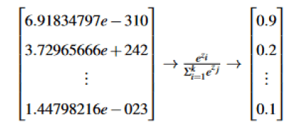
Linking different types of homologies to figure out the full simulation of persistent homology will be done using a training parameter under a reinforcement learning approach. We will be building neural networks using numpy library from python; with only two hidden layers our model seems to hide greater strategies in capturing alpha shapes from a twenty data set of matrices representing Hi as our training data set (Figure 9); to figure out probabilities we use the following softmax activation function [10].
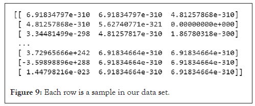
Figure 9: Each row is a sample in our data set.
pip install tensorflow biopython numpy pandas
import numpy as np
import pandas as pd
from Bio import PDB
def load_pdb_data (file_path):
parser = PDB.PDBParser()
structure = parser.get_structure (’protein’, file path)
atom_data = []
for model in structure:
for chain in model:
for residue in chain:
for atom in residue:
atom_data.append ([atom.get name (), atom.coord [0],
atomdf = pd.DataFrame (atom data, columns =[’AtomName’, ’X’, ’Y’,
return atom_df
#Example usage
pdb_data = load_pdb_data (’example.pdb’)
print (pdb data.head ())
# Data preparation
from sklearn.model_selection import train_test_split
from sklearn.preprocessing import StandardScaler
def prepare_data (df, labels):
features = df [[’X’, ’Y’,’Z ’]]. v a l u e s
s c a l e r = S t a n d a r d S c a l e r ()
f e a t u r e s = s c a l e r . f i t t r a n s f o r m (f e a t u r e s)
X _ t r a i n , X _ t e s t , y _ t r a i n , y _ t e s t = t r a i n _t e s t _ s p l i t (f e a t u r e s , l a b
return X _ t r a i n, X _ t e s t , y _ t r a i n , y _ t e s t
#Example labels (you would need actual labels for your dataset)
labels=np.random.randint (0, 2, len (pdb data)) # Example: Binary cl
X_train, X_test, y_train, y_test=prepare_data (pdb_data, labels)
#Define and train the model
import tensorflow as tf
from tensorflow.keras.models import Sequential
from tensorflow.keras.layers import Dense, Dropout
def build_model (input_shape):
model=Sequential ([
Dense (64, activation=’relu’, input_shape=(input_shape,)),
Dropout (0.5),
Dense (32, activation=’relu’),
Dense (1, activation=’sigmoid’)
])
model.compile (optimizer=’adam’,
loss=’binary_crossentropy’,
m e t r i c s =[ ’ a c c u r a c y ’ ])
return model
#Example usage
model=build model (X_train.shape [1])
model.summary ()
#Train the model
history=model.fit (X_train, y_train, epochs=10, batch_size=32, valid)
#Evaluate the model
loss, accuracy=model.evaluate (X_test, y_test)
print (f ” Test Loss: {loss}”)
print (f” Test Accuracy: {accuracy}”)
It was out of the scope of this proposition to deal theoretically with the use of statistical tests on the set of barcodes, but the application shows clearly that the method can surpass a simple statistical approach and instead of conducting a molecular dynamic simulation it is easier to use existing information from models to construct a quantified sequence of barcodes then to look for its convergence limit. We can find interesting productions in the literature but none exploited fully persistent homology far from being a statistical tool. An interesting attempt by using dynamical distances was made by Peter Bubenik and collaborators, but couldn’t theoretically justify barcodes as a statistical observation, instead it gives birth to a new functional tool which is persistent landscapes [17].
This work is providing a complete roadmap for persistent homology and application to protein structure design, prediction and analysis. Persistent homology is a powerful tool in the field of computational biology, allowing researchers to analyze complex biological structures with greater accuracy and efficiency. In order to fully understand the fundamental concept, the mathematical model is thoroughly explained. To get familiarized with the axiomatic idea, the full mathematical model is detailed, as already mentioned in the computational part and give a stochastically approval to our work but without getting in the details of the calculations and the theoretical justifications.
[Crossref] [Google Scholar] [PubMed]
[Crossref]
[Crossref] [Google Scholar] [PubMed]
[Crossref] [Google Scholar] [PubMed]
[Crossref] [Google Scholar] [PubMed]
[Crossref] [Google Scholar] [PubMed]
[Crossref] [Google Scholar] [PubMed]
[Crossref] [Google Scholar] [PubMed]
[Crossref] [Google Scholar] [PubMed]
[Crossref] [Google Scholar] [PubMed]
[Crossref] [Google Scholar] [PubMed]
Citation: Lamine Z, Mansouri MW, Mamouni MI (2024). A Mathematical Model for Protein Structure Prediction and Analysis. J Proteomics Bioinform. 17:673.
Received: 03-Sep-2024, Manuscript No. JPB-24-33809; Editor assigned: 05-Sep-2024, Pre QC No. JPB-24-33809 (PQ); Reviewed: 19-Sep-2024, QC No. JPB-24-33809; Revised: 26-Sep-2024, Manuscript No. JPB-24-33809 (R); Published: 03-Oct-2024 , DOI: 10.35248/0974-276X.24.17.673
Copyright: © 2024 Lamine Z, et al. This is an open-access article distributed under the terms of the Creative Commons Attribution License, which permits unrestricted use, distribution and reproduction in any medium, provided the original author and source are credited.