Journal of Geography  & Natural Disasters
Open Access

A Novel Methodology for Large-Scale Landslide Susceptibility Mapping Based on Landslide Domain; An Effective Tool for Local Landslide Management and Planning: A Case Study from Darjeeling Himalaya, India

Sumit Kumar^1*, Gargi Singh¹, Rabisankar Karmakar¹, Akshay Kumar Mishra¹, Mathiyalagan Rajkumar¹, Abhisek Kumar¹, Pankaj Jaiswal² and Saibal Ghosh^{1 *}Correspondence: Sumit Kumar, Geohazard Research and Management Centre, Geological Survey of India, Kolkata, India, Tel: +918794738224, Email:

Author info »

Introduction

Landslide susceptibility mapping is the measure of the likelihood of occurrence of landslide in an area on the basis of local terrain conditions [1] and is carried out worldwide in various scales ranging from regional (>100 sq. km) to catchment (10-100 sq. km) to slope (<10 sq. km) depending on three basic factors [2]: (i) Purpose of the study, (ii) Extent of the study area and (iii) Resources and data availability [3] which in turn affects the selection of the approach of mapping [2]. In general, the methods used for landslide susceptibility analysis at a regional or catchment scales are either statistical (bivariate or multivariate) or deterministic with qualitative or quantitative output. Most common statistical methods are Logistic Regression (LR), neural network analysis, data-overlay, index-based and Weight of Evidence analyses (WofE), with an increasing preference towards machine learning methods in recent years [4]. In these methods the input parameters are ranked based on expert opinion as in Analytic Hierarchy Process or weighted linear combination [5-9] or based on numerical correlation between the input parameters and landslides [10-13]. On the other hand, the deterministic approach is more site-specific or applied at a slope scale as the input parameters are highly site dependent and its parameterisation over large area is not trivial.

At a catchment scale, landslide susceptibility mapping is often carried out to provide input for landuse planning. The ideal choice of mapping here is large scale i.e., 1:10,000 or larger which can be used in decision making for planning risk mitigation options. The output can be either qualitative or quantitative, but more importantly is should provide information specific to the requirement. For example, for planning landslide mitigation options along a certain stretch of a road, it is important to have information on the type of slope failures expected from a given susceptible zone, their run-out susceptibility etc. in order to judiciously design economical mitigation measures. Although large-scale Landslide Susceptibility Maps (LSMs) are intended for better management of landslide hazard and risk, but world-over only a handful of literatures are available on the methodology for generating large-scale maps that can be useful to end users. Researchers have used bivariate (WofE) or multivariate (LR) statistical techniques using very limited thematic variables such as slope angle, Land Use and Land Cover (LULC) and Slope Forming Material (SFM) [14,15] or kinematic analysis [16] by using structural discontinuities or computing ‘Total Estimated Susceptibility Values (TESV)’ using rating and weights derived heuristically [17]. Ghoshal et al. have used Slope Mass Rating (SMR) in rocky slopes and shear strength parameters in overburden slopes to prepare a qualitative landslide susceptibility map on scale 1:10,000 [17]. In most case studies on large-scale LSM it is apparent that the output conveys the similar information as that of a catchment scale landslide susceptibility map. Only the difference is the size of individual mapping unit showing different susceptibility classes/probability values or in other word the largescale LSM is the zoomed-in of that of the catchment-scale LSM. Value-added information such as the type of landslide that can initiate from a given susceptible class, its inundation area, and type of failure as natural or anthropogenically induced is often not available in the maps.

One way to overcome these challenges is to prepare LSM specific for a given landslide type. However, such analysis requires high resolution input parameters and high density data coupled with intense field mapping. Nowadays, with the advent of very high resolution remote sensing data with sub-meter accuracy, high resolution Digital Elevation Model (DEM) with use of GIS-based modelling make it possible to prepare more user-friendly maps.

The landslide susceptibility not only include the landslide initiation zones, but also areas potentially affected by the traveling mobilized material [18]. Hence evaluation of initiation susceptibility and assessment of runout has been modelled by many workers [19-23]. Debris slide propagating into debris flows cause extensive damage in the lower reaches. The legacy data and analysis of landslide inventory shows that debris flow had caused extensive damage to the life and property in the Darjeeling area during the events of 2015 and September 2007 (source-Legacy data). Thus, a debris flow impact probability map was also essential to identify the vulnerable areas in conjunction with the debris flow initiation susceptibility.

In this research a more pragmatic landslide domain based approach has been introduced to define the landslide initiation susceptibility in respect to specific landslide process and type. Attempt has been made to optimise the selection of input parameters more relevant to define the stability condition of a given landslide type under the mapped geo-environmental conditions that are considered suitable for a large-scale (1:10,000) susceptibility mapping. For making it more user-friendly, in this research a debris flow run-out susceptibility map has been prepared to derive a holistic susceptibility condition of the study area. The output is in tune to the requirement of the land use planners and suffices the objective of a large-scale landslide susceptibility mapping.

Study area

The study area (Figure 1) is located in the south eastern part of Kurseong Subdivision, Darjeeling District, West Bengal, India, covering 30 sq. km and extends between Balasun and Chota Ringtong Rivers. The site was chosen because it is most vulnerable to landslide and pose high risk to infrastructure and population. Landsliding is common in the area during and after every rainfall-induced landslide event. Paglajhora sinking zone, a major sinking zone, is located within the study area. Besides, the study area has a national importance as the National Highways (NH55) and a UNESCO heritage site (the Darjeeling Himalayan railway line) pass through the area. Besides the physical risks, the geological mileau with a large lithological variation over this small area (from Siwalik Formation, Gondwana/Buxa Formation, Daling Group with Lingtse Gneiss intrusions, Paro Gneiss, Darjeeling/Kanchenjunga Gneiss etc,) and tectonic set up with the Main Central Thrust passing through the area [24]. The Main Boundary Thrust (MBT) passes near to the southern boundary of the area. The major part of the study area belongs to the Darjeeling gneiss of Higher Himalaya. Towards north and south of this gneissic rockmass different lithounits of Lesser and Sub Himalayan sequences are present. In the south, the rocks of Siwalik Group represented by grey coloured, salt and pepper textured sandstone, conglomerate, siltstone and shale of varying thickness exposed along the road cut and nala section starting from the foothills. Immediately north of the above sequence, a narrow belt of Gondawana sedimentary succession is exposed, comprising sandstone-quartzite, carbonaceous shale-slate, coal and conglomerate-pebbly slate association. Main Boundary Thrust (MBT) with the Siwalik Group of rocks separates the Gondawana sedimentary succession.

Figure 1: Location map of the study area
Note: Elevation: () High: 3559 m, () Low: 86, () Aol, () Roads

Further north, the Daling Group of rocks (low-grade pelite and psammopelitic rythmites with minor volcanic) is exposed. Further north, granite gneisses and high-grade meta-sediments belonging to the Central Crystalline Gneissic Complex (CCGC) are exposed over the low-grade metamorphics of the Daling Group as thrusted unit along the Main Central Thrust (MCT). Along the lower part of MCT, a strongly lineated, coarse to medium grained granite gneiss and granite mylonites (Lingtse gneiss) are found in the form of sheets exposed between Gayabari and 14th mile area. The area of study also encompasses part of two different basins. The geomorphology, geology, material on the slope, terrain parameters and the slope failures are controlled by such variation in lithological and structural disposition in the area.

Materials and Methods

Landslides are caused by interplay of different predisposing factors [25-28] and therefore their occurrences vary in space, time, magnitude and impact. Some of these factors are natural such as geology, slope angle and type, land cover, landform etc. while some are human-induced such as cut slope, removal of slope toe etc. Thus, interplay of these factors under appropriate climatic condition creates landslides that can be of variable magnitude and types within the similar mapped slope condition. This variation is due to many intrinsic natural factors such as localized changes in pore water pressure, rock-mass conditions, surface erosion etc. that are often not considered in a small-scale susceptibility mapping as these are not mappable at the given scale. However, combination of both intrinsic and extrinsic factors results in a landslide of a certain type, which can be accurately mapped and documented. In order to capture the predisposing factors of different landslide processes and determination of their instability conditions, the following approach has been used in this study as shown in Figure 2.

Figure 2: Logical framework of the landslide susceptibility modelling at slope scale

Landslide inventory

Historic information on landslide occurrences is considered as the fundamental part of the landslide susceptibility studies, which give shrewdness into the frequency, volumes, damage, and types of the landslide phenomena [29-31]. Therefore, landslide occurrences in the past and present are key to the future spatial prediction, threshold modelling and hazard and vulnerability analysis. A landslide inventory map provides the basic information for evaluating landslide hazards or risk and therefore is a prerequisite for such studies [30,32]. In this study, landslide inventory was prepared using multiple data sources, including high resolution earth observation of Cartosat-1 (2.5 m × 2.5 m), LISS IV (5.8 m × 5.8 m), Google Earth images and base satellite maps available in ESRI’s ArcGIS 10.3, Toposheets, railway slip register records, legacy data, local newspaper reports and internet blogs.

IRS P6MX LISS IV imagery (of 17.10.2006, 05.11.2006, 04.12.2006, 09.02.2008, 18.11.2008, 05.01.2010 and 18.03.2010 acquisition date) and Cartosat-1 Panchromatic imagery (2.5 m) are the two main sources used extensively in the course of the present study for preparation of landslide inventory.

Besides, a total 67 nos. of debris flows were mapped from different sources from within and nearby areas. Their source and run-out areas are separately mapped.

Figure 3 shows the spatial distribution of 180 landslide sources mapped within the study area. Most of the landslides are translational debris slides (146 no.s), followed by rock slides (24 no.s) and debris flows (10 no.s). A large number of landslides are located in the south-eastern part of the study area.

Figure 3: Landslide inventory map of the study area showing landslide source areas
Note: Landslide: () Debris flow, () Debris slide, () Rock fall, () Rock slide, () Road, () Drainage, () Location

A total 34 landslides are actually cut slope failures generated as a result of anthropogenic activity along road, railroad or at places within settlement area. These are small in size and mapped as point data.

Thematic variables

Landslide occurrences are influenced by interaction of a number of static and dynamic geo-factors. The selection of preparatory factors depends on the scale of study, the geo-environmental setting, the type of slope failures and their failure mechanisms [32,33]. van Westen et al. provided the list of all important geo-environmental factors required for landslide susceptibility analysis at different scales [34]. However, it is most important to select the optimal causative factors, out of the many commonly used factor maps which requires the prior knowledge about the causes of landslides in the area [35,36]. Based on the knowledge of the terrain and landslide occurrences Sarkar et al. used six thematic factors and Gogoi et al. used nine thematic maps such as DEM derivatives (slope, aspect and Curvature ) and categorical maps (Geomorphology, Land use/ land cover, Slope forming material, regolith thickness, drainage, structure) during the National Landslide Susceptibility Mapping (NLSM) [37,38].

Table 1 shows the determinant factors and data used for landslide susceptibility analysis. Another derivative maps that has been prepared in the scope of the study is engineering geology, kinematic failure and toppling failure map, which has been prepared through combination of field observations and analysis of geotechnical properties collected from representative slopes.

Table 1: Factors selected for landslide susceptibility analysis at slope scale

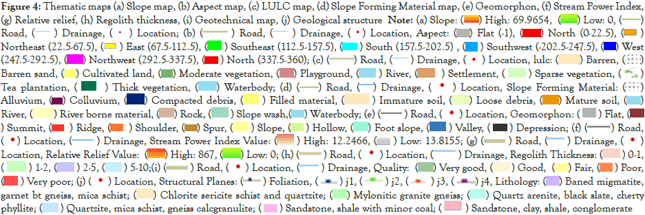
Slope map: Slope has a direct impact on landslide occurrences and is an important parameter in the landslide susceptibility analysis (Lee and Min, 2001). The slope map on 1:10000 scale is derived from CartoDEM as shown in Figure 4a.

Aspect map: Aspect define the direction of slope that has a direct bearing on the moisture content and vegetation; thus an important factor for slope stability. In Himalayas southerly facing slopes are directly exposed to monsoon activity, hence are favorable part of the slope facilitating mass movement. Sometimes penetrative structural elements control landsliding locally, following a certain aspect and thus the role of aspect become vital in controlling spatial distribution of landslide incidences and has a remote interrelationship with the geometry of the prevalent planar/linear structural fabrics of rockmass. The aspect map is divided into twelve (12) classes as shown in Figure 4b with 30 degree interval.

Land Use/Land Cover (LULC) map: Land Use and Land Cover (LULC) map shows the spatial distribution of most dynamic activity in the slopes. Vegetation plays a major role in resisting the slope movements due to root cohesion, particularly for failure with shallow slip/rupture surfaces [39]. Landslide susceptibility is affected by the presence or absence of vegetation. Thick vegetation reduces the absorption and evapotranspiration. Surface may be more or less prone to rill or gully erosion in relation to vegetation type. Stability of the slopes is increased by the root systems by increasing shear strength of soil through mechanical action and suction within the soil [40]. Besides, land use patterns like cultivation, urbanization and other anthropogenic activities also disturbs the natural equilibrium and affects the stability. Unscientific modification of slope also results in daylighting vulnerable planes, reducing toe support and/or loading of slope leading to destabilization. Anthropogenic activity and large-scale natural disasters change land use and landcover distribution of an area affecting the stability condition of the slopes. At slope scale more detailed information on LULC and its role in slope stability process was captured. Figure 4c shows the LULC maps of the study area.

Slope Forming Material (SFM) map: SFM is one of the principal governing factor in controlling the spatial distribution of landslides. The distribution of SFM units largely depends on underlying lithology, their degree of weathering and structural disposition, mass wasting history and sometimes anthropogenic intervention. It is an important static factor for causing landslides.

Figure 4d shows the slope scale (1:10,000) SFM maps of the study area prepared based on detailed field work. A total 22 different SFM classes have been identified. At slope scale the map could able, to capture more detailed information on SFM, of which few are significant in rendering slope unstable.

Geomorphon: The Geomorphon map is obtained by an automatic classification from a DEM. There are number of existing methodologies through which landforms can be prepared automatically by using the geo-morphometric variables [41-44], whereas manual classification involves recognition of whole topographic patterns corresponding to specific landforms. The manual process can bring in errors depending on experience and field knowledge of the terrain. The concept of geomorphon is based on the process of manual classification of landforms using the tools in computers to reduce human subjectivity. The geomorphon map have been prepared from 10 m × 10 m Cartosat- DEM for a 1:10,000 scale study area by using r.geomorphon script in GRASSGIS software.

Stream Power Index (SPI): The landslide occurrence near the stream in the study area shows that most of the debris and earth slide have occurred near the streams due to natural toe erosion. Erosion triggered by rainfall disturbs the slope equilibrium and causes landsliding [45], it was observed by Wistuba et al. [46] that landsliding and erosion, once triggered by precipitation, can occur alternately in years with average precipitation and reinforce one another. Stream Power Index (SPI) [47] is a tool to define the potential flow erosion at a given point of the topographic surface and has been widely used for landslide susceptibility mapping as shown in Figure 4e [48-52].

The SPI map as shown in Figure 4f is prepared using the raster calculator in Map algebra tool of ArcGIS 10.3.

Relative Relief (RR): The stability condition of material lying above the cut slope depends on the Relative Relief (RR) of the slope. For homegenous slopes with identical geomechanical and geometrical parameters, one having the higher elevation difference will be more susceptible to landslide [40]. These slopes will have higher runoff and lower infiltration [53]. Relative Relief (RR) is the variation in height calculated as the difference between the maximum and minimum heights in the terrain partitioning unit or slope unit [54] in the cut slope domain. The Relative relief as shown in Figure 4g of the slope unit is calculated using a zonal statistic function in ArcGIS 10.3. For the study area it varies from 0 to 867 m.

Regolith thickness map: The slope with higher regolith thickness is less stable at higher relief. “Regolith thickness” has been mapped to delineate the variation in the thickness of the units. The thickness is measured along the cut slopes, stream sections etc. The relatively small study area in 1:10,000 scale and available sections to measure the overburden depth with high certainty enables to map the regolith thickess as shown in Figure 4h.

Geotechnical/engineering geological map: The stability of a slope depends on the nature of material, its inherent disposition, shear strength, pore water pressure, groundwater regimes etc. The geotechnical properties of the soil/ overburden material and the slope mass ratings provide the basis for stability analysis of any rock/overburden material. This requires detailed mapping of the site and geotechnical properties of the rock and overburden. An engineering geological map speaks about the material properties that indirectly account for the pore pressure, rock mass character, infiltration etc. of the slope forming material. The slope forming material map hence is converted to the engineering geological map that represents the overall characteristic of the material based on the rockmass condition in rock outcrops and geotechnical properties of the overburden material.

The rocky slopes in the SFM map have been reclassified based on the rock mass condition (RMR_basic) [55]. For determination of RMR_basic, the field data on structures, orientation, properties like joint spacing, joint condition and hydrological conditions etc. along with geotechnical parameters of the rock samples such as specific gravity, density, void ratio, porosity, point load index determined in the laboratory has been used. The unconfined compressive strength of the rocks has been estimated in the field by using Schmidt hammer and has been corroborated with the point load index of the rock samples determined in the laboratory. The calculated RMR_basic at selected locations have been interpolated to other rocky slope units with similar disposition. The RMR_basic values as shown in Table 2 were categorized into the following four classes.

Table 2: RMR_basic classes after Bieniawski, Z.T. [55]

For the structural correction at each approachable rock exposure, the DEM derivative slope and aspect maps are used to prepare the geotechnical map of the rocky slopes. Figure 4i shows the geotechnical map of the study area at slope scale for all the six domains. The overburden slopes are classified based on the shear parameter of the material as shown in Table 3.

Table 3: Classification of overburden material based on shear parameters [17].

After the above classification relationship between slope and internal angle of friction were used [56] to further classify the map. Initially, the slope of each pixel/facet was subtracted from the friction angle. The higher values imply low susceptible zones and lower values imply high susceptible. Now the classified condition of overburden material according to Table 4 has been further degraded to lower category only if the area showing high to very high susceptible level according to the friction angle slope relationship as shown in Table 4.

Table 4: Susceptible condition based on the relationship between slope and friction angle [56].

The boundaries of the units were drawn based on the field exposures and the material characteristics. The very good to good category overburden material was found to be mainly restricted to the areas having matured soils and colluvium whereas as per their disposition at higher slope this material also falls in fair to poor category. The loose debris covered areas fall in very poor class and the slopewash material that occurs in major parts of the area falls in very poor to fair category. The immature soil also classed into a fair to poor category.

Geological structure: The stability of natural and man-made slopes is an important concern for numerous types of site uses and objectives, including the development or protection of infrastructure, settlements etc. Slope stability is largely dependent on the geologic and geotechnical characteristics of the bedrock that composes the slope. In rocky slopes, the most important factor is the geologic structure of the rock and the rock mass characteristic of the bedrock. Geologic structure refers to the location and orientation of the discontinuities within the bedrock mass and joint characteristics such as spacing, aperture, hydrological condition, Rock Quality Designation (RQD), strength parameter etc., refers to the rock mass characteristics of the bedrock. Such discontinuities include those along bedrock bedding/foliation, bedrock joints, faults, and shears.

The orientation and dip of structural data collected from the outcrops and from earlier work of Ghosh et al. were categorized using the stereoplot, [Stereonet (open source)] to identify the sets of discontinuities present in each slope [16]. A total of 367 no. of discontinuities data as shown in Figure 4j in the slope scale were used in the analysis which includes both the foliation and joint planes. Four major joint sets, namely J1 (southwesterly-dipping), J2 (southeasterly-dipping), J3 (northwesterly-dipping) and J4 (northeasterly-dipping) and foliation planes were mapped. Out of the total data, 135 nos. of foliation plane, 68 nos. of J1, 68 nos. of J2, 45 nos. of J3 and 52 nos. of J4 joint orientations were analyzed to assess the dominant orientation of these structures.

Mapping of landslide domain

Landslide domain represents areas having similar physiographic and geological characteristics that control the type of landslide occurring within it. It also helps in understanding the dominant landslide processes in the respective domain.

Landslide domains provide information on the types of landslide processes dominant within each domain which helps in optimizing the geo-factors responsible for rendering the slope unstable for a specific landslide type in an area. For example, orientation of the structural discontinuity plays a major role in stability in rock fall and rock slide domain than the debris slide or earth slide domain. Whereas, in the debris slide or earth slide domain the physical properties of the material and hydrological condition are dominant.

Criteria used for mapping landslide domain: The landslide domain map is prepared through two steps, (i) the domain with dominant material type and (ii) the domain with dominant landslide process.

For the preparation of landslide domain maps for dominant material type, slope forming material map is used as a proxy. From slope forming material map all the areas of overburden cover have been extracted assuming probable locale of debris slope failure and named as debris failure domain, likewise all areas of river, waterbody and alluvium were selected and named as no landslide domain. The alluvium material (sandy) is deposited within the river channel or at plain land and therefore these are grouped alluvium under no landslide domain. Moreover, all the areas with different rock cover are selected and named as rock failure domains. The areas covered with mature soil are classified into earth failure domains based on material characteristics (mostly fine and clayey). The material domains are subdivided into sub domains based on the expected dominant landslide processes and failure mechanism as guiding criterion to define the final landslide domains.

The rock failure domain in the areas of escarpment is selected and put under rock fall domain whereas, all the remaining areas of rock failure domain are selected and put under rock slide domain. All areas of debris failure domain with thickness less than 5 m are put under shallow translational debris failure domain and rest areas of debris failure domain with thickness more than 5 m as deep translational debris failure domain. Similarly, all areas of the earth failure domain with thickness less than 5 m are put under shallow translational earth failure domain and rest areas in earth failure and debris failure domain with more than 5 m thickness as deep translational earth/debris failure domain. In the study area as they are very small in size, hence they are merged with shallow merged with shallow translational earth/ debris failure domain.

As landslides are ubiquitous along the road sections the behaviour and factors also respond to the modification of the slope. Hence a domain named as cut slope failure domain is introduced. This domain was derived using the multiple buffers of the roads (NH, SH and other important roads where cut slope failure is active) and geomorphology. The no landslide domain are the areas where landside is not expected to like Rivers, waterbodies etc. Figure 5 shows the domain map of the study area mapped based on the criteria given above.

Figure 5: Landslide domain map of the study area
Note: Landslide domain: () Cutslope domain, () Shallow debris slide domain, () Shallow earth slide domain, () Rock fall domain, () Rock slide domain () No landslide domain, () Road, () Drainage, () Location

Selection of thematic variables

As the study area has been classified into different domains with dominant landslide process hence modelling of appropriate geofactors responsible for a specific dominant process is used. The selection of the geofactors for each domain was based on detailed study of the landslides of each type under different geo-environment settings. Landslide inventory highlights the typical character of landslides in the study area. Table 4 gives the controlling factors of the landslides as evidenced in the field and corresponding thematic variables mapped on 1:10,000 scale. The sub factors within each factor were also rated based on the potential contribution to slope failure as shown in Table 5. For example, a higher critical condition of kinematic failure (>5) will have a higher rating than a lower critical condition (1) in rock slide susceptibility. The resulting parametric equation is a sum, representing a Susceptibility Index (SI) or Total Estimated Susceptibility Values (TESV) ranging between 0 and 1 for each pixel (10 m by 10 m). After preparing the conditioning variable, each of the classes were ranked from 0-1 with an equal interval of 0.2 based on the importance. The Landslide Susceptibility Evaluation Rating (LSER) of the different classes of the variable responsible for landslides are given in Table 6. Table 7 gives the LSER of the various causative factors used in the modelling.

Table 5: Field and thematic variables responsible for landslide.

Table 6: LSER for various causative factors

Table 7: Maximum LSER ratings for various causative factors that affect stability of different domain at slope scale

The landslide susceptibility thematic mapping activity has been divided into five separate map products based on the five landslide processes of most frequent types in the area and the different factors responsible for causing these types of landslides. Five separate landslide susceptibility maps are prepared viz., rock fall, rock slide, debris slide, earth slide and cut-slope failure susceptibility maps. In each map, a series of thematic layers as shown in Table 5 was prepared i.e. geotechnical map, landuse/ landcover, regolith thickness or maps derived from DEM, i.e., slope angle and slope aspect, relative relief, stream power index and landform. From this information, a parametric equation was defined where the thematic layers served as variables with each variable being assigned a percent weight (LSER) based on expert knowledge. The resulting parametric equation is a sum, representing a Total Estimated Susceptibility Values (TESV) ranging between 0 and 1 for each pixel (10 m by 10 m). For the final map products, TESV were divided into three colour coded categories, low (green), moderate (yellow) and high (red) using Jenks natural breaks classification [57]. The landslide inventory was prepared as an independent variable used only for validation of the final susceptibility maps.

Semi quantitative heuristic method for rock slide and rock fall susceptibility

Rock related failures are mostly controlled by the orientation of the discontinuities and their interaction amongst themselves and the slope. In the study most of the rock slides were found to be caused by the interaction of joint planes and foliation plane. Kinematic analysis is mostly used to determine the potential modes of rock failure, and conventionally stereographic projection is used to determine this. In this method, the measured orientation of discontinuities are plotted on a stereonet and their stabilities are evaluated with respect to the slope orientation and friction angles of discontinuities [58]. Kinematic analysis uses Markland test [59] and has been employed for many kinematic analysis studies. The feasibility of specific discontinuity-controlled rock slope failure to occur at raster pixels can be spatially evaluated by simple first order kinematic criteria which determines the possibility of failure due to geometrical constraints [60,61]. The rigid failures of rock slopes along the pre-existing discontinuities can be identified by the relationship between the discontinuity attitude and slope angle [59]. Hence failure mechanism in each pixel was determined using kinematic analysis.

Kinematic analysis is based on the geometrical relationships between geologic structures and the orientation of overlying slopes. Therefore, to perform the analysis, both the topography (Slope angle(S) and Aspect (A)) and the attitude of geologic structure were considered across the area. The variation in slope orientation (i.e., slope angle and aspect) at local scale were evaluated using CartoSat Digital Elevation model of 10 m spatial resolution. DEM derived slope angle and aspect has been widely used in the slope stability analysis [16,62-65]. According to Hoek and Bray and Wyllie and Mah, when the discontinuity plane (for plane sliding) or intersection line (for wedge failure) of two discontinuities is shallower than the slope gradient but steeper than the friction angle of the discontinuities, failure occurs in the dip slope or oblique slope, respectively [60,66]. On the other hand, toppling failure occurs in the scarp slope when the discontinuity is parallel to a steep slope with an angle close to the dip direction of the structural discontinuity. Stereoplot is commonly used to check the above criteria by plotting the discontinuities and slope orientation. However, stereoplot is adequate for site-specific or single slope studies but at this type studies where rock slopes are widely distributed and topography is not uniform, the analysis becomes time consuming. So, to overcome this a GIS based approach is used to carry out the kinematic analysis at gridded raster pixel [16,66-69].

Application of kinematic analysis (kinematic modelling): The mean planar data of the foliation and joint planes (described in Thematic variables) was distributed in the whole area using the Inverse Distance Weighting (IDW) interpolation algorithm in ArcGIS 10.3 to generate the interpolated raster maps for dip and dip direction of each plane.

The planes for the prominent bedrock discontinuities derived using stereonets are given in Table 8.

Table 8: Mean plane orientation of the structural discontinuities

The total number of possible wedges formed by the intersection of any two discontinuity structural planes were derived with stereo plot of the discontinuities (Stereonet open source software). A total of 10 (Ten) conditions of intersection (trend and plunge) as shown in Figure 6 were identified and the trend and plunge of the identified intersection lines were interpolated by using IDW interpolation algorithm as shown in Table 9.

Figure 6: Stereo plot of the mean planar data and tier intersection points

Table 9: Intersecting lines attitude of the mean planes

The following raster layers were prepared for the structural parameters (trend and plunge of ten intersection lines and dip and dip direction of five planes).

• DIPj: Dip for each set of discontinuities.

• DIPDIRj: Dip direction for each set of discontinuities.

• IDIPi: Dip of intersection line between the sets of discontinuities.

• IDIPDIRi: Dip direction of intersection between the sets of discontinuities.

The suffixes j and i represent the sets of discontinuities and the intersections between them, respectively; therefore, j takes the values between 1 to 5 and i between 1 to 10.

Friction angle (Φ): The RMR system of Bieniawski was used for estimations of angle of internal friction (Φ). The empirical relationship between quality (Q) classification system and angle of internal friction (Φ) was estimated and used for each class in the geotechnical map as shown in Figure 4h [55]. Table 10 shows the value of angle of internal friction for each rock class.

Table 10: Friction angle and RMR relationship [55].

As per this system, the value of angle of internal friction is in the range of <15, 15-25, 25-35, 35-45 and >45. In the present study, the lowest value in the range is used assuming the worstcase scenario for stability conditions. The geotechnical map was rasterised using the Φ value using ArcGIS conversion tool, polygon to raster having cell size 10 m.

With the raster layers of the apparent dip, slope gradient and angle of internal friction, the possibility of kinematic failure (planar and wedge) in the rock slide domain and toppling failure mode in the rock fall [70] domain is evaluated in each pixel using raster calculator tool in map algebra of ArcGIS 10.3.

The apparent dip of the Discontinuity Plane (DIPj´) and the plunge amount (IDIPi´) in the slope direction were calculated using the Equations (ii) and (iii) respectively in raster calculator [66] of Map Algebra tool in ArcGIS to prepare fifteen raster maps of apparent dip and the plunge of the discontinuity planes for the study area.

DIPj´=Arctan (cos|Aspect-DIPDIRj|*tanDIPj) →Equation (i)

IDIPi´=Arctan (cos|Aspect-IDIPDIRi|*tan IDIPi) → Equation (ii)

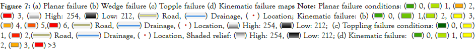
Planar failure: For planar failure to occur as shown in Figure 7a, the slope angle, the apparent dip (DIPj´) of the discontinuities and the friction angle (Φ) were used to derive the pixels critical for planar failure. If the apparent dip is less than the Slope angle (S) but greater than friction angle, the cell is identified as critical for planar failure [Equation (iii)]. In the rock slide domain out of the total 65283 pixels (10 m × 10 m), the equation satisfies conditions for one planar failure in 15234 pixels, two planar failure in 2188 pixels and three planar failure in 51 pixels. Rest pixels are free from any conditions for planar failure.

Plane failure: Φ<DIPj´<S → Equation (iii)

In ArcGIS 10.3 under the raster calculator tool under map algebra the following conditional statement is used to calculate the planar failure condition.

Con("friction.tif" < "DIP’.tif","DIP’.tif",99) and Con("DIP’.tif" < "slope.tif",1,0)

Wedge failure: For wedge failures as shown in Figure 7b, the derived plunge of the intersection between the discontinuity planes and slope are used to calculate daylighting conditions in the slope face.

To compare the slope angle to the plunge of intersection, apparent dip of the plunge (IDIPi´) in the slope direction is used where the apparent plunge of intersection is less than the slope angle but steeper than the friction angle, the cell is identified as critical for wedge failure [Equation(iv)]. In the study area out of the total 65283 pixels (10 m × 10m), the equation satisfied one wedge failure condition in 15799 pixels; two-wedge failure condition in 9245 pixels; three-wedge failure in 8481 pixels, 711, 42 and 1 pixels are observed to form 4, 5 and 6 wedge failure condition respectively.

Wedge failure: Φ<IDIPi´<S → Equation (iv)

In ArcGIS 10.3 under the raster calculator tool under map algebra the following conditional statement is used to calculate the planar failure condition.

Con("friction.tif" < "IDIP’.tif","IDIP’.tif",99) and Con("IDIP’.tif" < "slope.tif",1,0)

Toppling: Toppling failure occurs in scarp slope when the discontinuity is parallel to a steep slope with an angle close to the dip direction of the structural discontinuity and satisfies the Equation (v) as shown in Figure 7c.

Toppling failure: S ≥ Φ + (90°- DIPj´) → Equation (v)

In the study area out of the total 9360 pixels (10 m x 10 m) in the rockfall domain, the equation satisfied one toppling condition in 3798 pixels and two conditions in 1161 pixels. Rest pixels are free from any conditions for toppling failure.

Kinematic and toppling failure map: The kinematic failure map with total no. of critical condition for rockslide in each pixel was prepared by combining all the conditions for planar failure and wedge failure. Maximum eight critical conditions were identified in the rockslide failure domain in each pixel. It was reclassified into five classes having 0, 1, 2, 3 and >3 failure conditions. Figure 7d shows the spatially interpreted kinematic failure map integrating planar failure and wedge failure.

In this study to prepare a rock slide susceptibility map on a 1:10,000 scale, we propose a knowledge based model to characterize geologic structural controls on slope stability and the Geotechnical parameter of the rock.

As observed in the field, the most important ground conditioning parameters determining the occurrence of rockslides were the rock mass characteristic and the structural discontinuities. On this basis, a methodological framework was proposed for the rock slope susceptibility analysis at slope scale. The model was implemented in the study area by a procedure that comprises the following three parts: analysing the failure mechanisms of rock slide domain at the local scale, preparation of a geotechnical map and from this information, a parametric equation was defined where the data layers served as variables with each variable being assigned a percent weight based on expert knowledge. Classes within each layer of information were also rated based on the potential contribution to slope failure. The susceptibility was validated using the landslide data and the slope condition observed in the field.

The parametric equation used for the rock slide susceptibility map is:

TESV=0.6GT+0.4KF → Equation (vi)

Where variable GT is Geotechnical score map and KF is Kinematic Failure score map as shown in Table 6. KF only suggest the propensity of failure along a plane or wedge by virtue of the interaction of discontinuity planes at a given slope. It is observed in the field that the even though there are slopes with disadvantageous failure plains, still the rock mass is intact, which seem to be dependent on the inherent martial character in the slope. The geotechnical map that represents the material character such as parameters related to slope geometry, intact rock strength, discontinuity spacing or block size, hydrological conditions and shear strength along discontinuities etc. Higher weight is given to the geotechnical map than the kinematic failure map as the critical condition for kinematic failure, though is a prerequisite condition but inherent rock mass character defines the stability of the rock over the slope.

Rock falls strongly influence the evolution of steep rocky landscapes and represent a significant hazard in mountainous areas. Defining the most probable future rock fall source areas is of primary importance for susceptibility assessment. Thus, to understand which areas of a steep cliff are more likely to be affected by a rock fall, a semi quantitative heuristic method based on three factors viz., toppling failure condition, rock mass properties and landuse of the bedrock are used.

The parametric equation for rock fall susceptibility map is:

TESV=0.4GT+0.4TF+0.2LULC → Equation (vii)

In this method kinematic analysis was computed for toppling failure on vertical and overhanging rock walls according to the interaction between the discontinuities and the slope orientation. The classes of geotechnical map were assigned LSER similar to rock slide. In toppling failure higher rating were assigned to the maximum toppling condition observed in a pixel.

Qualitative heuristic method for debris and earth slide susceptibility

In order to prepare the susceptibility map of debris and earth slide, four factors viz. Stream Power Index (SPI), landform, LULC and GT map are used. Preparation and selection of these factors, such as SPI, LULC, GT and landform has been described in selection of thematic variables. All the maps are rasterised with a pixel size of 10 m × 10 m compatible with the spatial resolution of DEM.

The LSER of the SPI classes are given in Table 6. The higher rating is given to higher stream power index as higher SPI indicates more rill or gully erosion in the specific catchment and has direct impact on the stability of the slope.

These micro landforms are considered as an important factor closely related to landslide occurrence. The detailed landform map as shown in Figure 4d, consists of five prominent units such as flats, ridge-depression-valleys, shoulder-spur-footslope, Slope and Hollow. Hollow is the minor depression present in the slope which receives and contains high moisture or water. These are the initiation zone of most of the debris slide in the study area hence are given the highest rating whereas flats are given the lowest rating. The LSER of the landform classes are shown in Table 6.

Vegetation is a deterrent to erosion and improves the slope stability condition. The LULC map was reclassified into 5 five important classes as shown in Table 6 and high LSER is given to the thick vegetation cover and lowest to barren in debris and earth slide domain. Rest of the classes such as river, waterbody, settlement etc. are given 0 LSER as these classes are devoid of vegetation cover.

The angle of internal friction angle (∅), cohesion(c), slope and aspect are the most important properties of the overburden material that affect its stability. These parameters define the mechanical properties of the overburden. Geotechnical map of the overburden areas was prepared by using the mechanical properties of the material (Selection of thematic variables) and reclassified into five classes. The highest rating was assigned to very bad quality (1.0) and lowest rating was assigned to very good quality (0.2) based on their propensity to fail.

The parametric equation for the debris and earth slide susceptibility map is:

TESV=0.5GT+0.3LF+0.1SPI+0.1LULC → Equation (viii)

Where GT is Geotechnical map, LF is landform, SPI is Stream Power Index and LULC is landuse/landcover map. The Stream Power Index is (SPI) considered equally important as landuse/ landcover as vegetation cover and erosion are inversely related and low vegetation cover facilitate high erosion. Most of the debris slide in the area initiated near the streams at high slope having less vegetation cover. Geotechnical map has been given the highest LSER (0.5) rating as the engineering properties of the overburden material controls the stability of slopes in the area. Geotechnical map was derived from physical properties of the overburden material like friction angle, cohesion which are not variable and is a derivative of the measurement of its shear strength. It is a measure of the ability of a unit of overburden to withstand a shear stress.

Semi-quantitative and qualitative heuristic method for cut-slope susceptibility

The parametric equation used to prepare cut-slope failure susceptibility map is:

TESV=0.4 GT+0.2 RR+0.2 RT+0.2 S → Equation (ix)

Where, GT is Geotechnical map, RR is Relative Relief map, RT is Regolith Thickness map and S is the slope angle map. In the cut-slope failure domain Geotechnical map is considered to have maximum influence in initiating the cut-slope failures (as described in Thematic variables) and assigned a LSER of 0.4. Relative relief, Regolith thickness and slope angle are given equal importance based on field observation in cut-slope failure domain.

In the cut-slope domain, relative relief in the range 100-342 m covers nearly 56% of the area, while 44% of the area has low relative relief (0-100 m)). In the cut-slope domain 77% of the landslides are present in the highest relative relief range (>100 m) and 14% of the total landslide pixels are present in the range of 75-100 m, the rest are in the low relative relief range. Relative relief shows a positive spatial relationship with the landslides. Frequency distribution of landslides increases with increase in the relative relief.

Relative relief are divided into five classes viz., 0-25 m, 25-50 m, 50-75 m 75-10 m and more than 100 m. Maximum LSER (1.0) is assigned to highest class of RR i.e. more than 100 m and minimum LSER (0.2) to the lowest range of relative relief. Overburden material present on the higher relief becomes more unstable under the driving forces like gravitational pull in the slope above the formation. Similarly, in a cut slope, higher regolith thickness becomes more unstable at higher relative relief.

Debris flow susceptibility

Debris flow models are either complex physically based, mostly used in slope scale studies [71,72] or conceptual based used in catchment scale studies [73]. The conceptual models do not represent in detail the phenomena and physical processes of debris flows, but describe the behaviour of the flows based on simplified empirical relationships such as the angle of reach used for rock avalanches [73]; and debris flows [74,75]. In this study a conceptual model r.ramdomwalk based on source area definition and break criteria is used to prepare an impact probability map [76].

Debris flow map is prepared as a separate susceptibility map showing the probability of an area to be impacted by the movement of material while the landslide susceptibility map as discussed in material and methods shows the source zone and initiation of the landslides.

Input parameters and model calibration: Two input parameters essential for the modelling in the study area includes

• CARTO DEM of 10 m resolution is used to define the release pixels of the source areas.

• The debris flow inventory of 66 nos. of channelized debris flows polygons (Landslide inventory) were used to derive a statistical debris flow model.

For this, both the input parameters are used to calibrate the model for the identification of debris flow source areas and to define the stopping criterion/break criteria (or propagation distance) for debris flows.

Calibration of the conceptual model for modelling the propagation of debris flows: The r.randomwalk model [76] applied in the area to calculate the debris flow susceptibility. The stopping angle or angle of reach (ωT=Atan(H⁄L)) which is the the ratio between the difference in Height (H) and the distance travelled by the debris (L) that defines the criterion for defining the condition of stopping of the flows.

Results and Discussion

Figure 8a shows the landslide susceptibility map of the rock slide domain comprising 6.5 km² study area obtained using the parametric equation given in Equation vi as discussed in Semi quantitative heuristic method for rock slide and rock fall susceptibility. The rockslide susceptibility is reclassified into three classes using natural break [56] classification. The model could categorise about 28.81% area under high susceptibility (Probability >0.75) and spatially occur in the north-western part of the study area, downslope of Balasun and Margaret hope tea garden. Two infamous landslides in the past occurred in this part of the domain. The high susceptibility is also validated on ground as three planar failure and six wedge failure conditions prevail in the area due to the interaction between and foliation and joint. Few isolated patches are distributed throughout the domain area. Moderate susceptible zone covers about 32.8% of the domain area along the periphery surrounding the low susceptible slopes. The rock slide susceptibility classified the active rockslide zones in the extreme northern part of the domain area.

For Rock Slide domain susceptibility model output, the Probability >0.75 is considered as ‘unstable’ and rest as ‘stable’. The contingency table is obtained using 2707 pixels of selected landslide data set. Table 11 shows the confusion matrix of the output using LR method. The result indicates that the True Positive Rate (TPR) is 65.74% and over all accuracy of the model in defining stable and unstable zones is 72%. The model could able to characterise 65% of the selected source areas of mapped landslides within high susceptible zone (Probability >0.75) as shown in Table 11.

Table 11: Contingency matrix for the output of rock slide domain.

Figure 8b shows the landslide susceptibility map of the rock fall domain comprising 0.9 km² study area obtained using the parametric equation given in Equation (vii) as discussed in Semi quantitative heuristic method for rock slide and rock fall susceptibility. The rockslide susceptibility is reclassified into three classes using natural break [57] classification. The model could categorise about 11.9% of the rock fall domain area under high susceptibility (Probability>0.0.64) and are located in the northern part of the domain in the downslope of Balasun and Margaret hope tea garden in the steep escarpment slopes. The rock fall susceptibility classified the active rockfall zones in of the domain area as validated in the field. There was not any past rock fall inventory in the studied area to statistically validate the model.

Figures 8c and 8d shows the landslide susceptibility map of the debris slide domain comprising 15.8 km² study area and earth slide domain comprising 4.8 km² study area obtained using the parametric equation given in Equation (viii) as discussed in Qualitative heuristic method for debris and earth slide susceptibility. After preparing the debris slide susceptibility, it is reclassified into three classes using natural break [57] classification viz. low (0-0.6), moderate (0.6-0.76) and high (0.76-1). The debris slide model categorised about 38% of the debris slide domain area under high susceptibility (Probability >0.76) falling in the northern part of the domain in the eastern slope of Margaret Hope tea garden, upslope of Paglajhora, Giddapahar, western downslope of Gayabari and Tindharia villages. The presence of very bad quality of the overburden material and deep stream erosion in the upslope of Paglajhora River having many active subsidence zones, as observed in field, is classified as a large patch of high susceptible zone. Isolated patches of high susceptible zones are distributed throughout the study area. Moderate susceptible zone also covers about 36% of the study area surrounding the high susceptible areas. The model was able to classify 90 out of 106 landslides correctly in the high susceptible zone.

For Debris Slide domain susceptibility model output, the Probability >0.76 is considered as ‘unstable’ and rest as ‘stable’. The contingency table is obtained using 2117 pixels of selected debris slide data set. Table 12 shows the confusion matrix of the debris slide domain model. The result indicates that the True Positive Rate (TPR) is 65.74% and over all accuracy of the model in defining stable and unstable zones is 72%. The model could able to characterise 71% of the selected source areas of mapped landslides within high susceptible zone (Probability >0.75) as shown in Table 12.

Table 12: Contingency matrix for the output of debris slide domain.

The Susceptibility map of earth slide domain was classified as high (0.62-0.98), moderate (0.48-0.62) and low (0-0.48). In the Earth slide domain only 7.5% of the area is classified as highly susceptible and 44% of the area is classified as moderately susceptible. Most area under earth slide domain is stable under natural condition. The model could classify the area correctly as major part of the earth domain encompasses the ridge tops. There is no active or historical earth slide inventory in the study area to validate the model.

Figure 8e shows the landslide susceptibility map of the cutslope domain comprising 6.2 km² study area obtained using the parametric equation given in Equation (ix) as discussed in Semi-quantitative and qualitative heuristic method for cut-slope susceptibility. The slide susceptibility is reclassified into three classes using natural break [57] as low (0-0.52), moderate (0.52- 0.68) and high (0.68-1). The model could categorise about 44% of the cut slope domain area under high susceptibility (Probability >0.68) falling along NH-55 in the Geothel-Kariabasti, Kurseong viewpoint-Giddapahar, Tindharia-Chotta Ringtong sector. These are resulted due to excavation of hill slopes without following proper engineering standards and left exposed. The untreated slopes often initiate as small slope failures and develop into landslides of larger dimensions with passage of time.

Few high sporadic patches are also observed along the stream where active toe erosion is prevalent. Slope failures have also been reported along the drainages due to torrent streams leading to debris flow. These are more vulnerable in slopes comprising colluvial deposits and lying within 1^st and 2^nd order non-perennial drainages. Sudden heavy rainfall causes flow of material along such streams resulting in channelized debris flows.

For Cut-slope Slide domain susceptibility model output, the Probability >0.68 is considered as ‘unstable’ and rest as ‘stable’. The contingency table is obtained using 29 pixels of selected anthropogenic slide data set. Table 13 shows the confusion matrix of the cut-slope domain model. The result indicates that the True Positive Rate (TPR) is 86% and over all accuracy of the model in defining stable and unstable zones is 55%. The model could able to characterise 86% of the selected source areas of mapped landslides within high susceptible zone (Probability >0.75) as shown in Tables 13 and 14.

Table 13: Contingency matrix for the output of cut-slope domain.

Table 14: Gives the comparison of performance statistics of the rock slide, debris slide and cut-slope domain susceptibility models.

Figure 8f shows the impact Probability (P_I) map prepared from statistically derived cumulative density functions of the angle of reach from the 66 nos. of channelized debris flows. The PI ranges from 0-1, 0 being the low probability to be hit by the debris flows while 1 being the highest.

The impact probability was classified into five classes on natural break [57] in five break values, very low (0-0.22), low (0.22-0.48), moderate (0.48-0.63), high (0.63-0.78) and very high (0.78-1) probability. The debris flow susceptibility shows the area to be impacted by future debris flow events. The model captures the impact probability of the debris flow as is shown by the Figure 8f, wherein the available debris flow was superimposed over the debris flow impact probability map. It is seen that high impact area (red colour) shows the path of old debris flow occurrences in the area. The model has categorised 57% of the total area to be impacted by debris flow with 21% of the area having very high probability and 14% of the area with high probability. 65% of the total categorised debris flow susceptibility shows low to moderate impact probability. The high zones are distributed all over the study area and it shows the worst-case scenario for any unlikely event.

The larger aim of landslide susceptibility modelling under this research is to generate user friendly susceptibility maps to help the planners in mitigation and remediation. For making the model useable for decision support, it is of paramount importance that the landslide susceptibility map is of high quality, reliable and based on strong scientific basis coupled with validation.

Conclusion

The aim of this study is to present a methodology for landslide susceptibility mapping based on landslide process at slope scale (1:10000). It is observed that for a relatively small scale map (downscaling) requires more specific data on the landslide processes, to define the landslide susceptibility which requires domain specific analysis. As the preparatory factor maps need to convey the character of material (geotechnical properties) and structural disposition etc., hence geotechnical map, enhanced LULC, landform, SPI, relative relief maps became essential for a 1:10,000 scale susceptibility modelling. Landslide domains based on the landslide processes are defined and mapped as areas having similar physiographic and geological characteristics that controls the different type of landslide occurrence. Five landslide domain are prepared based on the processes namely, rock slide domain, rock fall domain, earth slide domain, debris slide domain and cutslope failure domain. For each domain, landslide process specific preparatory factors are identified and modelled separately for defining the susceptibility condition. A semi quantitative heuristic method is used after deriving parametric equations for each landslide domain based on the landslide preparatory factors and their role in landslide occurrence. Keeping in mind the user friendliness of the output maps, the susceptibility maps are generated with three susceptibility class viz. high, moderate and low.

The new technique for mapping the run out susceptibility (debris flow model) in both catchment and slope scale is prepared using the conceptual model “r.randomwalk”. The debris flow model is prepared by using the source zone break criteria (angle of reach) as input parameter and simulation of the source zone pixel following Monte Carlo approach. An impact Probability (P_I) map showing the area to be impacted by the future debris flow events is constructed. It is seen that high impact area (red colour) shows the path of old debris flow occurrences in the area. The debris flow run out model can be used in conjunction with an initiation susceptibility model to locate the high impact zones, however further research is required to find the way where both models can be combined together for generating a single map.

The validation of the maps with the landslide inventory shows that the overall accuracy of the rock slide susceptibility, debris slide susceptibility and cut-slope domain susceptibility are 0.72, 0.62 and 0.55 respectively. The susceptibility maps of earth slide and rock fall domains are not validated due to the non-occurrence of the landslide inventory. Besides, the slopes identified in field to be unstable also falls in high susceptible zones. It is concluded that downscaling of map do lead to better landslide prediction, however it requires intensive field input to derive the preparatory factors, mapping the discontinuities, defining the boundary of materials on the slope etc and laboratory inputs for preparing the geotechnical map.

It is concluded that the generated output of the susceptibility maps can be used by the stakeholders for management of landslide disaster at a local scale as a risk mitigation option.

Acknowledgements

The authors sincerely acknowledge the Director General, GSI; the Addl. Director General & Head: Mission IV, CHQ, and Deputy Director General, Mission-IVA, GSI, CHQ, Kolkata for allowing taking up this research work of great societal relevance. The authors are also indebted to the Shri Timir Ghosal, Director (Geology), EG and Landslide Division, GSI, Eastern Region, Kolkata for suggesting valuable technical comments to enhance the quality of the work.

The authors would also like to offer sincere gratitude to Dr. Ivan Marchesini of CNR-IRPI, Italy for their technical help in running the randomwalk tool.

Conflict of Interest

The authors have no known conflict of interest.

References

1. Brabb EE. Innovative approaches to landslide hazard and risk mapping. 1984.
2. Aleotti P, Chowdhury R. Landslide hazard assessment: summary review and new perspectives. Bull Eng Geol Environ. 1999;58:21-44.

   [Crossref] [Google Scholar]

3. Kanungo DP, Arora MK, Sarkar S, Gupta RP. Landslide Susceptibility Zonation (LSZ) Mapping–A Review. J South Asian Disaster Stud. 2009;2:81-105.

   [Google Scholar]

4. Reichenbach P, Rossi M, Malamud BD, Mihir M, Guzzetti F. A review of statistically-based landslide susceptibility models. Earth Sci Rev. 2018;180:60-91.

   [Crossref] [Google Scholar]

5. Yalcin A. GIS-based landslide susceptibility mapping using analytical hierarchy process and bivariate statistics in Ardesen (Turkey): comparisons of results and confirmations. Catena. 2008;72(1):1-12.

   [Crossref] [Google Scholar]

6. Komac M. A landslide susceptibility model using the analytical hierarchy process method and multivariate statistics in perialpine Slovenia. Geomorphol. 2006;74(1-4):17-28.

   [Crossref] [Google Scholar]

7. Ayalew L, Yamagishi H, Ugawa N. Landslide susceptibility mapping using GIS-based weighted linear combination, the case in Tsugawa area of Agano River, Niigata Prefecture, Japan. Landslides. 2004;1:73-81.

   [Crossref] [Google Scholar]

8. Akgun A, Dag S, Bulut F. Landslide susceptibility mapping for a landslide-prone area (Findikli, NE of Turkey) by likelihood-frequency ratio and weighted linear combination models. Environ Geol. 2008;54:1127-1143.

   [Crossref] [Google Scholar]

9. Ahmed B. Landslide susceptibility mapping using multi-criteria evaluation techniques in Chittagong Metropolitan Area, Bangladesh. Landslides. 2015;12(6):1077-1095.

   [Crossref] [Google Scholar]

10. Carrara A, Cardinali M, Detti R, Guzzetti F, Pasqui V, Reichenbach P. GIS techniques and statistical models in evaluating landslide hazard. Earth Surf Process Landf. 1991;16(5):427-445.

    [Crossref] [Google Scholar]

11. Guzzetti F, Reichenbach P, Cardinali M, Galli M, Ardizzone F. Probabilistic landslide hazard assessment at the basin scale. Geomorphol. 2005;72(1-4):272-299.

    [Crossref] [Google Scholar]

12. Jaiswal P. Landslide risk quantification along transportation corridors based on historical information. ITC. 2011.

    [Google Scholar]

13. Ghosh S, Carranza EJ, van Westen CJ, Jetten VG, Bhattacharya DN. Selecting and weighting spatial predictors for empirical modeling of landslide susceptibility in the Darjeeling Himalayas (India). Geomorphol. 2011;131(1-2):35-56.

    [Crossref] [Google Scholar]

14. Fressard M, Thiery Y, Maquaire O. Which data for quantitative landslide susceptibility mapping at operational scale? Case study of the Pays d'Auge plateau hillslopes (Normandy, France). Nat Hazards Earth Syst Sci. 2014;14(3):569-588.

    [Crossref] [Google Scholar]

15. Thiery Y, Malet JP, Sterlacchini S, Puissant A, Maquaire O. Landslide susceptibility assessment by bivariate methods at large scales: application to a complex mountainous environment. Geomorphol. 2007;92(1-2):38-59.

    [Crossref] [Google Scholar]

16. Ghosh S, Günther A, Carranza EJ, van Westen CJ, Jetten VG. Rock slope instability assessment using spatially distributed structural orientation data in Darjeeling Himalaya (India). Earth Surf Process Landf. 2010;35(15):1773-1792.

    [Crossref] [Google Scholar]

17. Ghoshal TB, Bodas MS, Ghosh S. A multi-thematic and deterministic-cum-heuristic methodology for mesoscale (1:5,000/10,000) landslide susceptibility zonation. Indian J Geosci. 2013;67(3):217-228.
18. Melo R, Zêzere JL. Modeling debris flow initiation and run-out in recently burned areas using data-driven methods. Nat Hazards. 2017;88:1373-1407.

    [Crossref] [Google Scholar]

19. Montgomery DR, Dietrich WE. A physically based model for the topographic control on shallow landsliding. Water Resour Res. 1994;30(4):1153-1171.

    [Crossref] [Google Scholar]

20. Dai FC, Lee CF, Ngai YY. Landslide risk assessment and management: an overview. Eng Geol. 2002;64(1):65-87.

    [Crossref] [Google Scholar]

21. Chung CJ, Fabbri AG. Validation of spatial prediction models for landslide hazard mapping. Nat Hazards. 2003;30:451-472.

    [Crossref] [Google Scholar]

22. Corominas J, Copons R, Vilaplana JM, Altimir J, Amigó J. Integrated landslide susceptibility analysis and hazard assessment in the principality of Andorra. Nat Hazards. 2003;30:421-435.

    [Crossref] [Google Scholar]

23. Hürlimann M, Copons R, Altimir J. Detailed debris flow hazard assessment in Andorra: a multidisciplinary approach. Geomorphol. 2006;78(3-4):359-372.

    [Crossref] [Google Scholar]

24. Dasgupta S, Ganguly J, Neogi S. Inverted metamorphic sequence in the Sikkim Himalayas: crystallization history, P–T gradient and implications. J Metamorph Geol. 2004;22(5):395-412.

    [Crossref] [Google Scholar]

25. Hungr O, Leroueil S, Picarelli L. The Varnes classification of landslide types, an update. Landslides. 2014;11:167-194.

    [Crossref] [Google Scholar]

26. Hungr O, Evans SG, Bovis M, Hutchinson JN. A Review of the classification of landslides of the flow type. Environ Eng Geosci. 2001;7:221-238.

    [Crossref] [Google Scholar]

27. Cruden DM, Fell R, 1997. Landslide risk assessment
28. Varnes DJ. Slope movement types and processes. Special Rep. 1978;176:11-33.

    [Google Scholar]

29. van Westen CJ, van Asch TW, Soeters R. Landslide hazard and risk zonation—why is it still so difficult?. Bull Eng Geol Env. 2006;65:167-184.

    [Crossref] [Google Scholar]

30. Regmi AD, Devkota KC, Yoshida K, Pradhan B, Pourghasemi HR, Kumamoto T, et al. Application of frequency ratio, statistical index, and weights-of-evidence models and their comparison in landslide susceptibility mapping in Central Nepal Himalaya. Arab J Geosci. 2014;7:725-742.

    [Crossref] [Google Scholar]

31. Youssef AM, Pradhan B, Jebur MN, El-Harbi HM. Landslide susceptibility mapping using ensemble bivariate and multivariate statistical models in Fayfa area, Saudi Arabia. Environ Earth Scien. 2015;73:3745-3761.

    [Crossref] [Google Scholar]

32. Guzzetti F, Carrara A, Cardinali M, Reichenbach P. Landslide hazard evaluation: a review of current techniques and their application in a multi-scale study, Central Italy. Geomorphol. 1999;31(1-4):181-216.

    [Crossref] [Google Scholar]

33. Glade T, Anderson MG, Crozier MJ. Landslide hazard and risk. Wiley. 2005.

    [Crossref] [Google Scholar]

34. van Westen CJ, Castellanos E, Kuriakose SL. Spatial data for landslide susceptibility, hazard, and vulnerability assessment: An overview. Eng Geol. 2008;102(3-4):112-131.

    [Crossref] [Google Scholar]

35. Ghosh S, Carranza EJ. Spatial analysis of mutual fault/fracture and slope controls on rocksliding in Darjeeling Himalaya, India. Geomorphol. 2010;122(1-2):1-24.

    [Crossref] [Google Scholar]

36. Ghosh S. Knowledge guided empirical prediction of landslide hazard. 2011:310-314

    [Google Scholar]

37. Sarkar NK, Ghosh S, Ghoshal T, Das S, Laskar T, Dattagupta T, et al. Macroscale Landslide hazard zonation in parts of Darjeeling district, West Bengal. Geol Surv India Unpub Report (FS 2003-05). 2005.

    [Google Scholar]

38. Gogoi D, Kavitha S, Kumar PK. Macro-scale (1:50,000) Landslide Susceptibility Mapping in parts of Toposheet nos. 78B/1, 5, 9,13 and 78A/16,Darjeeling and Jalpaiguri districts, West Bengal. 2016
39. Kuriakose SL. Physically based dynamic modelling of the effects of land use changes on shallow landslide initiation in the Western Ghats, Kerala, India. ITC. 2010.

    [Google Scholar]

40. Foumelis M, Lekkas E, Parcharidis I. Landslide susceptibility mapping by GIS-based qualitative weighting procedure in Corinth area. Bull Geol Soci Greece. 2004;36(2):904-912.

    [Crossref] [Google Scholar]

41. Evans IS. General geomorphometry, derivatives of altitude, and descriptive statistics. Routledge. 2019:17-90.

    [Google Scholar]

42. Pike RJ. The geometric signature: quantifying landslide-terrain types from digital elevation models. Math Geol. 1988;20:491-511.

    [Crossref] [Google Scholar]

43. MacMillan RA, Jones RK, McNabb DH. Defining a hierarchy of spatial entities for environmental analysis and modeling using Digital Elevation Models (DEMs). Comput Environ Urban Syst. 2004;28(3):175-200.

    [Crossref] [Google Scholar]

44. Olaya V. Basic land-surface parameters. Dev  Soil Scien. 2009;33:141-169.

    [Crossref] [Google Scholar]

45. Lévy S, Jaboyedoff M, Locat J, Demers D. Erosion and channel change as factors of landslides and valley formation in Champlain Sea Clays: The Chacoura River, Quebec, Canada. Geomorphol. 2012;145:12-18.

    [Crossref] [Google Scholar]

46. Wistuba M, Malik I, Wójcicki K, Michałowicz P. Coupling between landslides and eroding stream channels reconstructed from spruce tree rings (examples from the Carpathians and Sudetes–Central Europe). Earth Surf Process Landf. 2015;40(3):293-312.

    [Crossref] [Google Scholar]

47. Moore ID, Grayson RB, Ladson AR. Digital terrain modelling: a review of hydrological, geomorphological, and biological applications. Hydrol Process. 1991;5(1):3-30.

    [Crossref] [Google Scholar]

48. Pourghasemi HR, Pradhan B, Gokceoglu C. Application of fuzzy logic and analytical hierarchy process (AHP) to landslide susceptibility mapping at Haraz watershed, Iran. Nat Hazards. 2012;63:965-996.

    [Crossref] [Google Scholar]

49. Devkota KC, Regmi AD, Pourghasemi HR, Yoshida K, Pradhan B, Ryu IC, et al. Landslide susceptibility mapping using certainty factor, index of entropy and logistic regression models in GIS and their comparison at Mugling–Narayanghat road section in Nepal Himalaya. Nat Hazards. 2013;65:135-165.

    [Crossref] [Google Scholar]

50. Park S, Choi C, Kim B, Kim J. Landslide susceptibility mapping using frequency ratio, analytic hierarchy process, logistic regression, and artificial neural network methods at the Inje area, Korea. Environ Earth Sci. 2013;68:1443-1464.

    [Crossref] [Google Scholar]

51. Pradhan AM, Kim YT. Relative effect method of landslide susceptibility zonation in weathered granite soil: a case study in Deokjeok-ri Creek, South Korea. Nat Hazards. 2014;72:1189-1217.

    [Crossref] [Google Scholar]

52. Saadatkhah N, Kassim A, Lee LM. Susceptibility assessment of shallow landslides in Hulu Kelang area, Kuala Lumpur, Malaysia using analytical hierarchy process and frequency ratio. Geotechn Geol Eng. 2015;33:43-57.

    [Crossref] [Google Scholar]

53. Singh VP. Hydrologic systems: watershed modeling. Prentice Hall. 1988.

    [Google Scholar]

54. Alvioli M, Guzzetti F, Marchesini I. Parameter-free delineation of slope units and terrain subdivision of Italy. Geomorphology. 2020;358:107124.

    [Crossref] [Google Scholar]

55. Bieniawski ZT. Engineering rock mass classifications: a complete manual for engineers and geologists in mining, civil, and petroleum engineering. John Wiley Sons. 1989.

    [Google Scholar]

56. Roopnarine R, Eudoxie G, Opadeyi J. Soil friction angle as an instability factor in landslide susceptibility modeling. J Earth Scienc Geotech Eng. 2013;3(1):55-71.

    [Google Scholar]

57. Jenks GF. The data model concept in statistical mapping. Intern Yearb Carto. 1967;7:186-190.

    [Google Scholar]

58. Park HJ, Lee JH, Kim KM, Um JG. Assessment of rock slope stability using GIS-based probabilistic kinematic analysis. Eng Geol. 2016;203:56-69.

    [Crossref] [Google Scholar]

59. Markland JT. A useful technique for estimating the stability of rock slopes when the rigid wedge slide type of failure is expected. Imp Coll Rock Mech Res Rep. 1972.

    [Google Scholar]

60. Hoek E, Bray JW. Rock Slope Engineering. London: The Institution of Mining and Metallurgy. 1981.

    [Google Scholar]

61. Cruden DM. Limits to common toppling. Can Geotech J. 1989;26(4):737-742.

    [Crossref] [Google Scholar]

62. Derron MH, Jaboyedoff M, Blikra LH. Preliminary assessment of rockslide and rockfall hazards using a DEM (Oppstadhornet, Norway). Nat Hazards Earth Syst Sci. 2005;5(2):285-292.

    [Crossref] [Google Scholar]

63. Günther A, Wienhöfer J, Konietzky H. Automated mapping of rock slope geometry, kinematics and stability with RSS-GIS. Nat Hazards. 2012;61:29-49.

    [Crossref] [Google Scholar]

64. de Vita P, Cevasco A, Cavallo C. Detailed rock failure susceptibility mapping in steep rocky coasts by means of non-contact geostructural surveys: the case study of the Tigullio Gulf (Eastern Liguria, Northern Italy). Nat Hazards Earth Syst Sci. 2012;12(4):867-880.

    [Crossref] [Google Scholar]

65. Yilmaz I, Marschalko M, Yildirim M, Dereli E, Bednarik M. GIS-based kinematic slope instability and Slope Mass Rating (SMR) maps: application to a railway route in Sivas (Turkey). Bull Eng Geol Env. 2012;71:351-357.

    [Crossref] [Google Scholar]

66. Wyllie DC, Mah C. Rock slope engineering. CRC Press. 2004.

    [Google Scholar]

67. Günther A, Carstensen A, Pohl W. Automated sliding susceptibility mapping of rock slopes. Nat Hazards Earth Syst Sci. 2004;4(1):95-102.

    [Crossref] [Google Scholar]

68. Kim KS, Park HJ, Lee S, Woo I. Geographic Information System (GIS) based stability analysis of rock cut slopes. Geoscien J. 2004;8:391-400.

    [Crossref] [Google Scholar]

69. Aksoy HÜ, Ercanoglu MU. Fuzzified kinematic analysis of discontinuity-controlled rock slope instabilities. Eng Geol. 2007;89(3-4):206-219.

    [Crossref] [Google Scholar]

70. Günther A, Carstensen A, Pohl W. Automated sliding susceptibility mapping of rock slopes. Nat Hazards Earth Syst Sci. 2004;4(1):95-102.

    [Crossref] [Google Scholar]

71. Christen M, Bartelt P, Kowalski J. Back calculation of the In den Arelen avalanche with RAMMS: interpretation of model results. Ann Glaciol. 2010;51(54):161-168.

    [Crossref] [Google Scholar]

72. Christen M, Kowalski J, Bartelt P. RAMMS: Numerical simulation of dense snow avalanches in three-dimensional terrain. Cold Reg Sci Technol. 2010;63(1-2):1-14.

    [Crossref] [Google Scholar]

73. Adrian ES. On the prediction of the reach and velocity of catastrophic landslides. Rock Mech. 1973;5(4):231-236.

    [Crossref] [Google Scholar]

74. Zimmermann M. Murganggefahr und Klimaänderung-ein GIS-basierter Ansatz. Vdf Hochs AG. 1997.

    [Google Scholar]

75. Rickenmann D. Empirical relationships for debris flows. Nat Hazards. 1999;19:47-77.

    [Crossref] [Google Scholar]

76. Mergili M, Krenn J, Chu HJ. r. randomwalk v1, a multi-functional conceptual tool for mass movement routing. Geosci Model Dev. 2015;8(12):4027-4043.

    [Crossref] [Google Scholar]