Journal of Theoretical & Computational Science
Open Access
ISSN: 2376-130X
ISSN: 2376-130X
Research Article - (2014) Volume 1, Issue 2
The B-factor, also called the Debye-Waller factor or the temperature factor, is a descriptor of the flexibility of protein and is commonly used in PDB (Protein Data Bank) format files. A B-factor could be measured from a protein crystal by x-ray scattering, but could not be got from the protein sequence directly. Thus, predicting the B-factor only based on the protein sequence could provide some references for the related researchers. In this study, we attempt to predict the B-factor based on the protein sequence. The information in AAindex and the predicted protein secondary structure, relative accessibility, disorder and energy changes are used to describe the amino acid residues. Four machine learning methods are used for modeling and prediction. The 5-fold cross validation is used to evaluate the modeling performance. As a result, this work provided some new methods for predicting and analyzing the B-factor based on the protein sequence, and we hope that this work could be helpful for the related researches.
<Keywords: B-factor, Protein sequence, Machine learning, Regression, Random forest
The Debye-Waller factor [1] is used to describe the attenuation of x-ray scattering or coherent neutron scattering due to the thermal motion. The Debye-Waller factor is also called the B-factor when measuring the flexibility of protein structure. The B-factor could be obtained by the formula:
B factor = 8π2 (μ2)
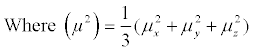
The μx, μy, and μz represent the atomic displacements from the three coordinate axes. In a PDB (Protein Data Bank) [2] format file, every atom has a B-factor in the ATOM records, and the B-factor of a residue is the average of the B-factors of all the atoms that constitute this residue. The residues with low B-factors commonly have a stable structure and the ones with large B-factors are generally more flexible. The protein flexibility and B-factor act an important role in the research of the molecular recognition, catalytic activity, allosteric and evolution [3-7]. Hence, the research of B-factor could be help for the development of the related fields.
On the other hand, the available records of the protein sequences are far more than the ones of the protein structures. For example, the number of the records in the Uniport is more than 1,386,943 [8], but the number of the entries in the RCSB Protein Data Bank is about 84,000 [2]. Thus the information based on the protein structure is still less than the information from protein sequence. Therefore, using protein sequence to speculate the information of the structure is always a research hotspot. For example, the Critical Assessment of Structure Prediction (CASP) experiment [9] is held periodically to find some models to predict the 3-D structure from the protein sequences. Using the sequence to predict the B-factor is complicated because of the lack of information that could link to the displacements of the protein atoms. A common way is to find the similar sequences that have the 3-D structure by using the sequence alignment tools such as BLAST [10] and ClustalW [11], then using some machine learning and statistical methods to generate a model for the prediction of the information of the residues. For example, Pan et al. [12] used the PSSM (position-specific scoring matrix) [13,14] and some other properties, such as the physicochemical properties, to predict the B-factor through a two stage support vector regression (SVR) [15].
In this study, we attempt to predict the B-factor based on the protein sequence. 107,322 residues from 474 protein chains constitute the training and test datasets. The properties in the AAindex and the predicted information of the secondary structure, relative accessibility, disorder and mutation energy change are used as the attributes of the datasets. Four machine learning methods, such as the random forest regression and liner regression, are used to predict the B-factor. All the predicting results are listed in the tables in the result section for discussion and comparison. The modeling and predicting results could be used as a reference for the related research.
In this study, the work flow is described in Figure 1, and the details are listed in the subsections respectively.

Figure 1: The workflow of this study.
Dataset
Based on the previous works [12,16], the two datasets in this study, PDB196 and PDB290, are used. Each protein chain in the two datasets has more than 80 residues, and the sequence similarities among the protein chains are less than 25%. Besides, according to the records in the PDB format files, the resolutions of the protein crystal are less than 2Å, and the R-factors are less than 0.2. Because of the update of the Protein Data Bank, some proteins are removed by some reasons such as the overlap or redundancy with other entries. The related ids are: 1191, 1531, 1alo, 1gdo, 1hal, 2ilb, luae, lxgs, lycc, 1eqo, 1hlr, 1uox. After taking out the absent entries, totally 64,844 residues from the PDB290 are used as the training dataset, and 42,478 residues from PDB196 are used as the test dataset.
Descriptors
The descriptors are used to generate the attributes of the residues in the datasets. In this study, the disorder, mutation information, secondary structure, relative accessibility, physicochemical and biochemical properties are used. With these descriptors, 1105 (1 + 40 + 2 + 531 * 2) attributes are generated for modeling. The related attributes are generated by the tools or resources respectively: DISpro, MUpro, SCARTH and AAIndex.
DISpro
The DISpro [17] is a software which could predict the disorder regions of an amino acid sequence by the 1D-RNNs (1-D recursive neural networks) [18], and could give each residue a value to measure the probability of disorder. The residues in the disorder regions are generally partially or wholly unstructured and do not fold into a stable state, and would be more flexible. Therefore, in this study, the probability values are used as an attribute of the dataset.
Mupro
The ability of the mutation from a residue to another could reflex the flexibility of the tested residue in some degree. The Mupro [19] could predict the value of energy (Gibbs free energy) change and the affection of a mutation by using the support vector machine (SVM). Being similar with the PSSM [13,14], both the energy changes and affections could be represented as 20 attributes which are consisted with the 20 natural amino acids.
SCARTH
The SCARTH [20] is a web server which could predict some properties of protein. In addition, a free desktop version is provided and could predict the protein secondary structure and the relative solvent accessibility. The second structure could be predicted as 8 classes (Table 1).
| Name | H | G | I | E | B | T | S | C |
|---|---|---|---|---|---|---|---|---|
| Explanation | alpha-helix | 310-helix | pi-helix | extended strand | beta-bridge | turn | bend | the rest |
Table 1: The explanations of the predicted secondary structure from the SCARTH.
The relative solvent accessibility could be predicted into 20 classes which represent the thresholds from 0% to 95%. For example, if the predicted value of a residue is 65, it means the relative solvent accessibility of this residue is ranging from 65% to 70%.
Different secondary structures could have disparate structure flexibilities, and the relative solvent accessibility is correlated with the environment of a residue. The two attributes would be related to the structure flexibility. In this study, the information of the second structure and relative solvent accessibility are used as 2 attributes of the datasets.
Attributes from AAIndex
AAindex: AAindex [21] is a database of numerical indices representing various physicochemical and biochemical properties of amino acids and pairs of amino acids. We think that some physicochemical and biochemical properties might be correlated to the B-factor, thus the information in AAIndex1 (a part of AAindex) is used for the amino acid residues. In this study, the indexes in AAindex1 are used for the residues. Some indexes which contain incomplete value (such as the value of residue P is NA in the index with the header AVBF000101) are ignored. Finally, 531 indexes are used to generate the attributes. Besides, the values of the residues would be reassigned in consideration of the affection from the adjacent residues.
Reassign the values via the residue contact network
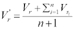
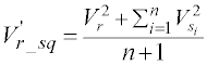
Considering that the residues in a protein chain would be affected by some adjacent residues, the values of the residues from the AAIndex1 were reassigned through the amino acid contact network (Figure 2).

Figure 2: The reassignment via the amino acid residue contact network.
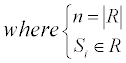
For a residue r, assume a set R={s | s is in contact with r} to represent all the contacted residues of r, the new value of r could be represented by the average value:

Besides, the squared values are also used as the attributes:
Through the network, the affection from the adjacent residues could be contained. Besides, because that only the protein sequences are used, the residue contact networks are generated by the software SELECTpro [22], which could predict the protein contact network based on the protein sequence.
The standardization of the values
All the values, including the B-factor, are standardized according to the formula:
The μ is the average value of an attribute and the σ is the unbiased estimation of the variance.
Machine learning methods
Four machine learning methods are used to mine the datasets in order to build a satisfactory model for the prediction of the B-factor. Besides, considering that the indexes from AAindex might be redundancy, a variable selection method is used to reduce the number of the attributes.
Select the attributes
The proportion of the number of residues and attributes is about 97:1. This proportion means that the instances (residues) are plenty for modeling by the machine learning methods. But the redundancy of the attributes still might affect the performance of the modeling results. In order to reduce the redundancy and find the best attributes which are related to the B-factor, the variable selection method is used to reduce the dimension of the attributes.
In this study, the variable selection method is the ReliefF [23] in the data mining toolbox WEKA [24]. ReliefF could evaluate each attribute and give it a value, then the attributes could be ranked by these values. With the generated rank list, the number of the attributes is shrunk into 5, 15, 30, 50, 100 and 300. Moreover, all the modeling output are compared and listed in the Table 3.
Modeling methods
The linear regression, REP Tree, Gaussian Process regression and Random Forest regression are used to predict the B-Factor. Considering the memory usage and modeling efficiency, the machine learning software WEKA [24] and Waffles [25] is utilized. The linear regression and REP Tree are from WEKA, and the other two regression methods are from Waffles.
Moreover, the secondary structure is used as a pseudo-variable when modeling. Both WEKA and Waffles support the attribute which is consists of some classes and would convert this attribute into the pseudo-variable automatically.
In this section, the modeling results would be provided and discussed.
Evaluation criteria
The CC (Correlation Coefficient), RMES (Root Mean Squared Error), MAE (Mean Absolute Error), RAE (Relative Absolute Error), RRSE (Root Relative Squared Error) are used to evaluate the prediction outputs. The formulas are as follows:
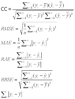
Where the n means the number of the instances, the y means the measured value, the  means the predicted value, and the
  and
and  mean the average values of the measured and predicted values.
The selected attributes
The algorithm ReliefF could rank the attributes by its inside evaluation mechanism. The first 10 attributes and the corresponding evaluated values are listed in Table 2.
| Ranking Number | Attribute Name | Evaluated value |
|---|---|---|
| 1 | Secondary Structure | 0.07575077 |
| 2 | Relative Solvent Accessibility | 0.04544955 |
| 3 | Disorder | 0.01861623 |
| 4 | WERD780103 (squared)of AAindex1 | 0.00969653 |
| 5 | QIAN880115 (squared) of AAindex1 | 0.00832180 |
| 6 | NAKH900110 (squared) of AAindex1 | 0.00764229 |
| 7 | QIAN880126 (squared) of AAindex1 | 0.00764118 |
| 8 | QIAN880114 (squared) of AAindex1 | 0.00724505 |
| 9 | QIAN880128 (squared) of AAindex1 | 0.00692809 |
| 10 | TANS770102 of AAindex1 | 0.00691166 |
Table 2: The first 10 selected attributes.
Table 2 demonstrated that the first 3 attributes are most important for modeling according to the evaluated values. Besides, the squared value from AAindex1 is also useful. The descriptions of the selected AAindex headers in Table 2 are: Free energy change (WERD780103), weights for beta-sheet (QIAN880***), normalized composition of membrane proteins (NAKH900110) and normalized frequency of isolated helix (TANS770102).
Table 2 also implies that the B-factor is mainly correlated with the structure and physicochemical information, thus the related attributes, such as the Secondary Structure, Relative Solvent Accessibility, disorder and weights for beta-sheet, are selected by the ReliefF.
The prediction results
The results are listed in the Table 3. The best value of each criterion is marked as bold.
| Var Num | Methods | Performance of Training dataset | Performance of Independent Test dataset | ||||||||
| CC | RMSE | MAE | RAE | RRSE | CC | RMSE | MAE | RAE | RRSE | ||
| 5 | Liner regression | 0.4549 | 0.8905 | 0.6341 | 0.8749 | 0.8906 | 0.4577 | 0.7680 | 0.5664 | 0.9163 | 0.9021 |
| Gauss Process | 0.4472 | 0.9451 | 0.6779 | 0.9353 | 0.9452 | 0.4438 | 0.8036 | 0.6173 | 0.9987 | 0.9940 | |
| REP Tree | 0.4545 | 0.8933 | 0.6346 | 0.8756 | 0.8934 | 0.4103 | 0.8051 | 0.5904 | 0.9551 | 0.9457 | |
| Random Forest | 0.4820 | 0.8764 | 0.6236 | 0.8605 | 0.8765 | 0.4342 | 0.7833 | 0.5750 | 0.9302 | 0.9201 | |
| 15 | Liner regression | 0.4643 | 0.8857 | 0.6288 | 0.8676 | 0.8858 | 0.4645 | 0.7672 | 0.5665 | 0.9164 | 0.9012 |
| Gauss Process | 0.4361 | 0.9010 | 0.6400 | 0.8831 | 0.9011 | 0.4435 | 0.7930 | 0.5882 | 0.9515 | 0.9315 | |
| REP Tree | 0.4699 | 0.8844 | 0.6248 | 0.8620 | 0.8845 | 0.4221 | 0.7978 | 0.5877 | 0.9508 | 0.9371 | |
| Random Forest | 0.5858 | 0.8318 | 0.5840 | 0.8058 | 0.8318 | 0.4385 | 0.7725 | 0.5697 | 0.9216 | 0.9075 | |
| 30 | Liner regression | 0.4697 | 0.8829 | 0.6257 | 0.8634 | 0.8829 | 0.4698 | 0.7655 | 0.5641 | 0.9125 | 0.8992 |
| Gauss Process | 0.4335 | 0.9021 | 0.6396 | 0.8825 | 0.9022 | 0.4390 | 0.7995 | 0.5909 | 0.9559 | 0.9392 | |
| REP Tree | 0.4676 | 0.8892 | 0.6241 | 0.8611 | 0.8863 | 0.4209 | 0.7987 | 0.5877 | 0.9507 | 0.9382 | |
| Random Forest | 0.6015 | 0.8283 | 0.5815 | 0.8023 | 0.8284 | 0.4150 | 0.7816 | 0.5767 | 0.9330 | 0.9182 | |
| 50 | Liner regression | 0.4697 | 0.8829 | 0.6258 | 0.8634 | 0.8829 | 0.4698 | 0.7655 | 0.5641 | 0.9125 | 0.8992 |
| Gauss Process | 0.4271 | 0.9139 | 0.6497 | 0.8964 | 0.9141 | 0.4306 | 0.8426 | 0.6195 | 1.0022 | 0.9898 | |
| REP Tree | 0.4736 | 0.8822 | 0.6214 | 0.8574 | 0.8823 | 0.4124 | 0.8086 | 0.5926 | 0.9586 | 0.9498 | |
| Random Forest | 0.5964 | 0.8285 | 0.5813 | 0.8021 | 0.8286 | 0.3917 | 0.7901 | 0.5833 | 0.9436 | 0.9281 | |
| 100 | Liner regression | 0.4697 | 0.8828 | 0.6257 | 0.8634 | 0.8829 | 0.4698 | 0.7655 | 0.5641 | 0.9126 | 0.8992 |
| Gauss Process | 0.4219 | 0.9197 | 0.6519 | 0.8995 | 0.9198 | 0.4240 | 0.8543 | 0.6269 | 1.0142 | 1.0035 | |
| REP Tree | 0.4784 | 0.8793 | 0.6194 | 0.8546 | 0.8794 | 0.4091 | 0.8130 | 0.5957 | 0.9637 | 0.9550 | |
| Random Forest | 0.5948 | 0.8289 | 0.5804 | 0.8008 | 0.8290 | 0.3646 | 0.7998 | 0.5911 | 0.9562 | 0.9395 | |
| 300 | Liner regression | 0.4696 | 0.8829 | 0.6258 | 0.8634 | 0.8830 | 0.4698 | 0.7655 | 0.5641 | 0.9125 | 0.8992 |
| Gauss Process | 0.4116 | 0.9149 | 0.6490 | 0.8956 | 0.9150 | 0.4109 | 0.8241 | 0.6110 | 0.9884 | 0.9681 | |
| REP Tree | 0.4787 | 0.8796 | 0.6186 | 0.8535 | 0.8798 | 0.4703 | 0.8144 | 0.5912 | 0.9564 | 0.9567 | |
| Random Forest | 0.5996 | 0.8256 | 0.5783 | 0.7979 | 0.8256 | 0.3639 | 0.8003 | 0.5912 | 0.5964 | 0.9401 | |
| all | Liner regression | 0.4703 | 0.8838 | 0.6263 | 0.8620 | 0.8829 | 0.4630 | 0.7697 | 0.5668 | 0.9221 | 0.9083 |
| Gauss Process | 0.3885 | 0.9317 | 0.6570 | 0.9066 | 0.9318 | 0.3988 | 0.8359 | 0.6183 | 1.0002 | 0.9819 | |
| REP Tree | 0.4739 | 0.8825 | 0.6202 | 0.8557 | 0.8826 | 0.4233 | 0.7967 | 0.5880 | 0.9513 | 0.9538 | |
| Random Forest | 0.4880 | 0.8732 | 0.6212 | 0.8572 | 0.8732 | 0.4469 | 0.7787 | 0.5717 | 0.9249 | 0.9148 | |
Table 3: The predicting results.
The Table 3 illustrates that the random forest could train a model that is fit for the training dataset, but the predicting performance of the test dataset is relatively unsatisfactory. On the other hand, the linear regression, a fundamental algorithm, shows a stable performance on both modeling and prediction. Moreover, the prediction results are similar when the number of used attributes exceeds 30, and the best prediction performances are concentrated where the number of the attributes is 30.
The comparisons between the measured and predicted values are provided in Figure 3. The used dataset in Figure 3 is the independent test data, and the used models are the ones which have the best training performance in Table 3. Moreover, considering of the large scale of the dataset, only 500 samples are randomly selected for this plotting. Besides, the 4 subfigures are provided separately as the supplementary.

Figure 3: The comparison between the measured and predicted values.
As an empirical result, if the distributions of a dataset in the sample space and feature space are adequate, the modeling results from the adapted methods would be similar. In this study, the number of the instances is abundant, thus the ‘dimensional disaster’ could be avoided and the fundamental algorithm, such as the linear regression, could get a stable predicting performance. However, according to the Table 3, the distribution of the training dataset and test dataset in the sample space might be not so consistent. Thus the predicting result of the model from random forest is not satisfactory. To verify this assumption, the training dataset and test dataset are combined into a large dataset, and the Random Forest with the 5-fold cross validation are used in modeling and validating. Moreover, to confirm the stability of the prediction, the inner 5-fold cross validation is utilized. The result is in Table 4.
| Var Num | Cross validation (inner/outer) | Performance of Training dataset | ||||
|---|---|---|---|---|---|---|
| CC | RMSE | MAE | RAE | RRSE | ||
| 5 | inner1 | 0.4651 | 10.1162 | 7.2018 | 0.8693 | 0.8855 |
| inner2 | 0.4684 | 10.1391 | 7.1953 | 0.8672 | 0.8837 | |
| inner3 | 0.4681 | 10.0993 | 7.1854 | 0.8687 | 0.8839 | |
| inner4 | 0.4646 | 10.1212 | 7.1967 | 0.8700 | 0.8857 | |
| inner5 | 0.4655 | 10.1357 | 7.2052 | 0.8702 | 0.8853 | |
| outer | 0.4692 | 10.1052 | 7.1783 | 0.8668 | 0.8833 | |
| 15 | inner1 | 0.5559 | 9.6909 | 6.7923 | 0.8199 | 0.8482 |
| inner2 | 0.5546 | 9.7411 | 6.7971 | 0.8192 | 0.8490 | |
| inner3 | 0.5580 | 9.6846 | 6.7783 | 0.8195 | 0.8475 | |
| inner4 | 0.5528 | 9.7142 | 6.7863 | 0.8204 | 0.8501 | |
| inner5 | 0.5574 | 9.7036 | 6.7913 | 0.8202 | 0.8475 | |
| outer | 0.5653 | 9.6396 | 6.7350 | 0.8133 | 0.8426 | |
| 30 | inner1 | 0.5675 | 9.6735 | 6.7625 | 0.8163 | 0.8467 |
| inner2 | 0.5648 | 9.7334 | 6.7691 | 0.8158 | 0.8483 | |
| inner3 | 0.5688 | 9.6707 | 6.7520 | 0.8163 | 0.8463 | |
| inner4 | 0.5644 | 9.6995 | 6.7587 | 0.8171 | 0.8488 | |
| inner5 | 0.5686 | 9.6900 | 6.7604 | 0.8165 | 0.8463 | |
| outer | 0.5787 | 9.6069 | 6.6955 | 0.8085 | 0.8397 | |
| 50 | inner1 | 0.5546 | 9.7149 | 6.7959 | 0.8203 | 0.8503 |
| inner2 | 0.5513 | 9.7787 | 6.8099 | 0.8208 | 0.8523 | |
| inner3 | 0.5551 | 9.7201 | 6.7899 | 0.8209 | 0.8507 | |
| inner4 | 0.5525 | 9.7366 | 6.7939 | 0.8213 | 0.8520 | |
| inner5 | 0.5556 | 9.7331 | 6.7987 | 0.8211 | 0.8501 | |
| outer | 0.5682 | 9.6381 | 6.7287 | 0.8125 | 0.8424 | |
| 100 | inner1 | 0.5643 | 9.6711 | 6.7409 | 0.8137 | 0.8465 |
| inner2 | 0.5579 | 9.7510 | 6.7563 | 0.8143 | 0.8498 | |
| inner3 | 0.5637 | 9.6803 | 6.7365 | 0.8144 | 0.8472 | |
| inner4 | 0.5606 | 9.7010 | 6.7381 | 0.8146 | 0.8489 | |
| inner5 | 0.5636 | 9.6955 | 6.7415 | 0.8142 | 0.8468 | |
| outer | 0.5760 | 9.5959 | 6.6652 | 0.8049 | 0.8387 | |
| 300 | inner1 | 0.5551 | 9.6912 | 6.7585 | 0.8158 | 0.8483 |
| inner2 | 0.5483 | 9.7728 | 6.7785 | 0.8170 | 0.8517 | |
| inner3 | 0.5538 | 9.7031 | 6.7618 | 0.8175 | 0.8492 | |
| inner4 | 0.5496 | 9.7298 | 6.7611 | 0.8174 | 0.8515 | |
| inner5 | 0.5523 | 9.7276 | 6.7643 | 0.8170 | 0.8496 | |
| outer | 0.5662 | 9.6215 | 6.6852 | 0.8073 | 0.8410 | |
| all | inner1 | 0.5147 | 9.9085 | 6.9437 | 0.8381 | 0.8673 |
| inner2 | 0.5077 | 9.9881 | 6.9640 | 0.8393 | 0.8705 | |
| inner3 | 0.5148 | 9.9088 | 6.9445 | 0.8396 | 0.8672 | |
| inner4 | 0.5095 | 9.9408 | 6.9462 | 0.8397 | 0.8699 | |
| inner5 | 0.5113 | 9.9471 | 6.9554 | 0.8400 | 0.8688 | |
| outer | 0.5255 | 9.8525 | 6.8823 | 0.8311 | 0.8612 | |
Table 4: The predicting results from the combined dataset by using Random Forest.
The results from Table 4 could verify the assumption that the distribution of the two datasets are not very consistent. The Random Forest algorithm would build many trees by random sampling, thus the distribution of the sample space would affect the predicting result. The differences between the Table 3 and Table 4 indicate that the kind of the data in the training dataset could be extended.
Besides, according to the selected attributes in Table 2, the values of the disorder, relative accessibility and secondary structure are most important and are relative to the B-factor. It is obvious that the value of B-factor depends on different structure, but the predicting results imply that the relationship between the B-factor and the secondary structure might be simple so that the fundamental linear regression could get good predicting results. The predicting results from Random Forest also imply this point.
The comparison with other works
There are some similar works which were proposed by other researchers. The related details are provided in the Table 5.
| Methods | CC on Training Dataset | CC on Independent test |
|---|---|---|
| Gumbel distribution [16] | 0.34 | 0.37 |
| Vihinen’s methods [16] | 0.31 | 0.33 |
| Karplus and Schulz ’s methods [16] | 0.30 | 0.33 |
| NS [26] | 0.34 | - |
| KS [26] | 0.38 | - |
| PS [26] | 0.41 | - |
| 2-stage SVR [12] | 0.53 | 0.55 |
| This worka | 0.60 | 0.41 |
| This work (combination)b | 0.57 | 0.58 |
athe results are from the method with the best CC value on training dataset in Table 3, e.g. the Random Forest with 30 attributes
bthe results are from the Random Forest with 30 attributes in Table 4. The CC values on training dataset is the average CC values of the five inner folds, and the CC value of the independent test is the related outer folds
Table 5: The comparison with other works.
Since only the CC values are provided in the previous works, more detailed comparison, such as the comparison among the RMSEs, could not be provided. The other evaluation criteria would be useful and could reflect some properties in some situations. For example, according to the Table 3, the values of RMSE and MAE from the predicting results are generally better than the ones from training dataset, but the others are not. It might be caused by the difference of the  in the formula of RAE and RRSE. If the
  or
or  is larger, the values of RAE and RRSE would become smaller relatively, thus even though the predicted value is more close to the measured one, the RAE and RRSE would not be smaller because of the low variance of the B-factor values. This situation could reflect that the distributions of the B-factor among the training dataset and test dataset are different in some degree, and more samples are needed for modeling.
In this study, we use some predicted information of the protein structure based on the sequence and the indexes from AAindex to predict the B-factor. Four machine learning methods are used to mine the dataset, and finally we get the similar prediction results with other previous works. The used attribute is mainly related to the structure, physicochemical properties and biochemical properties, which might be more correlated to the B-factor. However, all the used attributes need to be generated from some machine learning model, and the predicted information would increase the noise of the dataset and decrease the performance of the final prediction. For example, we think that the reassignment via the contact network might be helpful for the adjustments of the attributes. However, the SELECTpro could only generate the contact network of the residues, thus the distances between two residues are missing and the cut-off threshold and the weighted reassignment could not be considered into this study. This limited situation would be improved through the rapid increase of data and the development of machine learning theory in the future.
Besides, using protein sequence to predict the information based on the structure is a long-standing challenge. With the statistical methods, this challenge could be addressed in some extent. The evolution relationships among the query sequences and the alignment dataset could be generated through the sequence alignment tools, then the relationships could be used to link the sequences to some known structures. With the links, the needed information could be generated through some machine learning and statistical methods. In this study, we used more than one machine learning methods to predict the B-factor, and employed five criteria to assess the prediction results. We hope that this study could provide more information to the researchers in the related fields and could be useful for the researchers.
We would like to thank the anonymous reviewers for their patient review and constructive suggestions. This work was supported by the National Natural Science Foundation of China (21375090).