Proteomics is the large scale study of proteins in order to obtain a global, integrated view of disease processes, cellular processes and networks at the protein level. In contrast to traditional approaches that examine one or a few proteins at a time, proteomics attempt to examine large numbers of proteins concurrently. Mass spectrometry (MS) has been successfully applied to the analysis of protein/peptide and has become the workhorse of proteomics in the last few years (Aebersold and Mann, 2003). A mass spectrometer takes a molecular mixture as input and determines the mass of the molecules, or, more precisely, their mass over charge ratio, m/z. The output of mass spectrometer is referred to as a spectrum. Ideally, a feature in a mass spectrum indicates the presence of molecules of the corresponding m/z value in the sample, while the height of the feature is referred to as the observed intensity y. However, both the m/z values and the intensities y’s are influenced by confounding factors.

Mass spectrometry (MS) for the protein analysis consists of diverse technologies and techniques e.g. Matrix-assisted laser desorption/ionization-time of flight (MALDI-TOF), Surfaceenhanced laser desorption/ionization-time of flight (SELDI-TOF) etc. Although, reproducibility of the data is in question for different mass spectrometry platforms, there are many works relating to identification of proteomic biological markers using mass spectrometry (Petricoin et al., 2002a, b, c, d; Wulfkuhle, 2003; Zhu et al., 2003). (Diamandis, 2003, 2004a, b, c) revealed that proteomic biomarkers are more specific and sensitive than others, even though there are many challenges when detecting them. Till today, discovery of biomarkers using automatic analysis of proteomics mass spectra is still growing.

One of the first steps of analyzing mass spectrum is to detect true signals or peaks from contaminated features (Mantini et al., 2007; Morris et al., 2007). Most peak detection algorithms simply identify peaks based on their amplitude. The performance of a peak detection method directly affects the subsequent process, such as possible biomarker identification of a protein (Noy and Fasulo, 2007). Unlike peak detection using amplitude, monoisotopic peak detection is simply detecting a unique peak for each peptide. Monoisotopic peak means the mass of the peptide if no heavy isotopes are involved. Because of their uniqueness, most of the peptide mass finger printing (PMF) techniques use monoisotopic peaks to identify proteins. Thus, it is important to precisely determine the monoisotopic peak from a collection of features.

Algorithms which detect monoisotopic peaks usually consider the probable isotopic distributions of peptide molecules within a spectrum. So far only the Peak Harvester developed by (Breen et al., 2000, 2003) can automatically detect monoisotopic peaks using a mixture of location-shifted Poisson distribution to model the isotopic distributions of the peptide molecules. However, the parameter estimation of the Poisson distributions in their case involves substantial assumptions derived from the prior knowledge in the protein sequence database. We modify the procedure of parameter estimation to be a data driven approach instead of a database approach. In our method, parameters of the location-shift mixture Poisson models are estimated using maximum likelihood method with Expectation Maximization (EM) technique, and the behavior of the EM estimators proposed is studied numerically through Monte Carlo simulations.

The structure of this paper is as follows: In Section 2, we discuss the methods employed for preprocessing, extraction of isotopic distribution, model fitting, and checking the adequacy of the fitted model along with testing for monoisotopic peaks. We describe the simulation study for showing the adequacy of the parameter estimation through power and size calculation in Section 3. Section 4 contains a real data analysis example and relative performance of our method with another recent method of peak detection. Section 5 contains discussion and more details about future work.

Data Preprocessing

As data preprocessing could severely affect the outcome of the monoisotopic peak detection, all steps in data preprocessing should be carefully evaluated. A volume of work has been done on preprocessing, e.g. ( Breen et al., 2002; Breen et al., 2003) used interpolation techniques and mathematical morphology for the detection of important features or peaks. Including the work of Wu et al., (2003) on background noise reduction, Satten et al., (2004) for standardization and denoising the MALDI-MS spectra, Malyarenko et al., (2005) for baseline correction etc. Coombes et al., (2005) and Morris et al., (2005) used wavelets for noise reduction. Sauve and Speed, (2005) used a mathematical morphological filter to denoise a spectrum followed by dynamic programming to align multiple spectra. Mantinni et al., (2007) used a Kaiser digital moving window filter to obtain smoothed signal, then subtracted a signal trend for baseline removal. Once the baseline removal was completed, a local maxima is used to find the most significant peaks after eliminating the features with intensities lower than a non-uniform threshold proportional to the noise level. Then, the detected peaks are classified as either protein or noise peaks on the basis of their m/z values. In this paper, a different preprocessing approach is proposed to identify regions of interest.

Our preprocessing of MALDI-TOF data involves two steps: baseline correction and denoising. The process converts each spectrum into stick representation where each stick corresponds to a denoised and baseline corrected peak. Our baseline correction relies on a method proposed by Li, (2001) and noise removal which is based on our proposed method. Li, (2001) have written a number of software routines to handle mass spectrometry data and have combined them into R Package, PROcess which is available from http://www.bioconductor.org. The routine, bslnoff, in the PROcess package is used to remove baseline drift from the spectrum. The function bslnoff divides the spectrum into unequal sections, find a minimum or a quantile corresponding to given probability of each section, replace each intensity by that minimum and fits a curve through all points.

Although the spectra after baseline correction have a common scale and fair homoscedasticity, they still contain a mixture of noise and signal. So, we denoised all the spectra. A cutoff point (h) is chosen such that the features selected correspond to real m/z peaks. The cutoff should be large enough to eliminate the initial noisy region but small enough to retain any peaks that could correspond to real observable proteins or peptides. The principle is based on keeping the features with intensities greater than certain threshold , where is the indicator function, the main advantages of this denoising process is very simple, do not require any model fitting and very fast. Another critical point in that we do not need to transform the intensities of the remaining peaks.

Isotopic Distributions

Isotopes are atoms of the same element with the same atomic number (number of electrons or protons) but with different atomic masses due to presence of different number of neutrons. For example, two naturally occurring carbon isotopes are C₁₂ and C₁₂. Both isotopes are exactly the same except that C₁₂ has 6 neutrons, while C₁₃ has 7 neutrons. As a result, their atomic masses are 12 and 13.0033 unified atomic mass unit (mu), or dalton (Da), is a unit of mass used to express atomic and molecular masses, respectively. The successive isotopic elements of a peptide molecule are commonly 1 (Da) apart. On the other hand, the monoisotopic peak is formed from the lowest- mass stable isotope of each element (i. e. all carbons are C₁₂, all nitrogens are N₁₄ , all oxygens are O₁₆ and all sulphers are S₃₂ etc.) and has a unique element composition, whereas other isotopic peaks include contributions from different elemental combinations (e.g., two C₁₃ vs. two N₁₅ vs. one C₁₃ and one N15, etc., at ~2 (Da) higher in mass than the monoisotopic mass). Because of the uniqueness of the monoisotopic peaks, most peptide mass fingerprinting (PMF) techniques used them to identify proteins by matching their constituent fragment masses (peptide masses) to the theoretical peptide masses generated from a protein or DNA database.

Considering the high influence of the isotopic distribution on finding the monoisotopic peaks, a new scheme is proposed for extracting the isotopic distribution of peptides. Our scheme works as follows: Assume that contiguous peaks x or m/z of 1Dalton (Da) apart exist in a isotopic distribution and that a is taken as starting value for identifying a isotopic distribution pattern in a spectrum. We make sure that there are no peaks to the left of a within 1 ± .05 Da, where .05 is the error tolerance (Breen et al., 2003) due to limitations of mass resolution. We can identify a isotopic distribution by selecting the peaks at a, a + 1 ( ± .05), a + 2 ( ± .05),… and we stop if a gap exists. The gaps exist when the distance between two consecutive peaks is greater than 1(± .05) Da.We kept repeating this procedure and form all possible isotopic distribution patterns in the spectrum. Before extracting the isotopic distribution, some binning is applied to reduce the data because spectrum data are very large. Our binning scheme works as follows: we round all the m/z values and within 1Da interval of each m/z, we keep the one corresponds to the maximum value of the intensity y.

Model Fitting

A isotopic distribution of any mass peptide can be modeled using binomial expansion (McCloskey, 1990). However, as the number of total atoms n of a specific type is large compared to the relative abundance of the isotope p, one can fit a Poisson distribution to model a isotopic distribution (Breen et al., 2000, 2003). However, overlapping distributions of resolved peaks can happen due to deamidation (Breen et al., 2000). Deamidation is a process that some proportion of an amino acid N or Q gets converted to D or E respectively. The change results in an increase of 1Da in the mass of the peptide molecule that carries the modified amino acid caused by the replacement of NH. groups from N or Q with OH groups from D or E. So, there will be a shift to the isotopic distribution. As the deamidation of a peptide makes the isotopic distribution of a peptide into two super imposed signals, a mixture of location-shifted Poisson is fitted to model each of the deamidated (possibly) isotopic distribution.

(Breen et al., 2000, 2003) utilized existing database knowledge to establish a linear equation between M the mean of a Poisson distribution and the peptide’s molecular weight m which is known. To do that, an average amino acid (AA) C₁₀H₁₆N₃O₃ is constructed by averaging all AAs from all proteins in the SWISS-PROT database. To cover a mass range from m₁ = 245.1376 Da to m₁₅ = 3410.8059 Da, multiples of the average AA are used. For each constructed theoretical peptide with mi:i = 1,…15, the isotopic distributions are calculated using protein Prospector. The mean M_i is found by minimizing the sum absolute deviation between the components of distributions. As a result, the mean M can be calculated from the following equation M = .000594m− .03901. Using this linear equation, they computed expected heights of peaks in a spectrum and decided (in a somewhat ad hoc or non-statistical manner) whether the observed peaks can correspond to a series generated by a peptide. Since the regression line depends on the composition of the database whose coverage could change over time and may not be reliable in all cases; in addition, the resulting method may not be robust with respect to a change in the operational parameters of the mass spectrometry experiment.

The main advantage of our method over (Breen et al., 2000, 2003) is that we are not required to make use of any external knowledge for estimating the parameter values of the model. The parameters of interest are all local to a given spectra which are estimated using a statistical estimation technique (maximum likelihood). Furthermore, a call is subsequently made based on a statistical significance test of goodness of fit. Thus, our method is simpler (no operational or tuning parameters to select other than the threshold stage), automatic and statistically well grounded.

The proposed mixture model in our paper fitted to a collection of adjacent features {y (x ): x=a+i, i=0 …i^*_a } at low to moderate molecular weight of peptides approximates the (relative) intensity distribution with that of a probability histogram corresponding to a mixture of two location-shifted Poisson distributions, y(x) / T = f_λ1λ2,w(i) + O_p(1), with

is the sum of the intensity values and a is the starting value of the isotopic pattern; the o_p (1) term converges to zero in probability as T gets large. Learning the mixture, namely estimating the weight and the parameters λ_j: j =1, 2 of each Poisson distribution, is carried out through likelihood maximization using the EM algorithm (Dempster et al., 1977; McLachlan and Krishnan, 1977). We present a methodology which involves the representation of the mixture problem as a particular case of maximum-likelihood (ML) estimation when the observations can be viewed as complete data. The ML method is so far the most widely used method of estimation. The associated efficiency and the well-understood properties of the ML estimates are well accepted. Previously, the computational difficulties in deriving the ML estimates had led the researches to use different estimation. However, nowadays the impact of computer intensive methods resulted in a very large number of applications based on ML estimation.

The Score Equations for Estimating the Model Parameters

Suppose that we have a random sample X₁, X₂, …, X_T where each X corresponds to the respective m/z value a+i in a isotopic distribution and has a probability function P_λ1λ2w given by (1). We do not actually observe the individual X but rather the histogram of X which would represent part of a spectrum displaying a monoisotopic pattern. However, as shown later, this does not pose a problem for parameter estimation and statistical inference since all the procedures will be based on the grouped data (histogram) that forms a set of sufficient statistics for this model.

The log-likelihood function l of this sample is:

where w₁ =w,w₂ =1−w are the mixing proportions and f(x | λ_j ) = I(x ≥ 0) e^-λ_jλ_j^x / x!, is the Poisson probability mass function with parameter λ_j, j=1,2.

In order to find the maximum likelihood estimators, we set up the score equations by equating all the partial derivatives of l with 0 solving them simultaneously:

Finding a simple analytical solution for these equations is not possible and the need for numerical methods is obvious. Newton Raphson method can be used in such cases. However, the applicability of this method becomes harder in multidimensional settings. The slow speed and lack of convergence guaranty are known issues with this method. Often an iterative synchronization scheme such as the Expectation Maximization (EM) algorithm (Dempster et al., 1977) is used to solve score equations. We now describe how to use the EM algorithm in this specific context.

Details of the EM Algorithm for a Mixture of Locationshifted Poisson Model

EM algorithm is originally designed for likelihood problems with “missing data”. In our context of fitting a mixture model, the group level indicators G can be considered to be missing. More specifically, let for each X_k as described above, G_k denotes which component (first or second) of the mixture distribution (1) generated X_k. The EM procedure iteratively maximizes Q(θ | θ^m, x) = E(l(θ | X, G) X = x, θ^m where θ^m = (λ₁^m, λ₂^m, w^m) is the current value of the parameters at step m where l(θ |X, Y)is the full data log-likelihood

The iteration θ^m —> θ^m+1 is defined through the following:

1. E-step: Compute Q(θ | θ^m, x)

2. M-step: θ^{m + 1} = argmax_θ€Φ Q(θ | θ^m, x).

By direct calculation we can show that the parameter estimates updating scheme in this problem is given by :

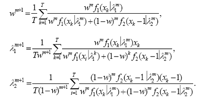
Note that these expressions can be written in terms of the available grouped data { y(x) : x = a + i, i = 0, … , i_a^* } representing the intensities of features separated by one Da

Choosing the initial values and convergence criterion are also taken into consideration when implementing the EM algorithm. Following one of the methods described by Karlis and Xekalaki, (2003) , the initial values are taken to be:w =5,

λ₁ = max { x^- - [ ( s² - x^- + ½ ) ]^½, 0.01 },

λ₂ = x^- - 1 + [ ( s² -x^- + ½ ) ]^½,

where x^- is the mean and s² is the variance of the grouped data x with frequency y(x), for x = a + i, i=0, …, i_a^*. These formulas are slightly different from the ones stated in Karlis and Xekalaki, (2003) since the second Poisson component is location shifted. These are basically the method of moments estimates of λ₁ and λ₂ assuming w = 0.5. The iterative EM procedure is stopped when max { | w^m+1 - w^m |, |λ₁^m+1 - λ₁^m |, | λ₂^m+1 - λ₂^m | } < 10^-4.

Checking the Adequacy of Model Fit

After fitting the above mixture model to a collection of adjacent features or binned clusters of features { y(x): x = a + i, i= 0…i_a^* }, we check the adequacy of the model fit by a bootstrap test. In particular, we conduct the following tests of hypotheses to determine the existence of a isotopic pattern and consequently designate a monoisotopic peak.

Testing the Isotopic Pattern

We consider the problem of testing the goodness of fit of a location shifted Poisson model applied to the intensity values of a cluster of adjacent m/z values separated by 1 Da. More formally, the null hypothesis we are testing is that

H₀₁: The intensities y(x) The intensities x = a + i, i= 0…i_a^* follow a mixture of location-shifted Poisson model f(|w, λ₁ λ₂) given by (1).

To this end, we propose four omnibus tests, using the Kullback-Leiber (KL) distance (Kullback and Leibler, 1951; MacKay, 2003), the Hellinger distance (Eslinger et al., 1995; Karlis and Xekalaki, 1998), the Kolmogorov- Smirnov (KS) supremum distance (Chandra, 1997) and the L₂ distance (MacKay, 2003). The basic idea behind each of these tests is to compare the estimates of the probability mass functions obtained from model (1) with their empirical (nonparametric) counterparts. Statistical significance of each of these test is determined by p-values computed using a parametric bootstrap scheme.

If H₀₁ is rejected, then we conclude that the above collection of adjacent features does not follow a isotopic pattern and hence does not contain a isotopic peak. Generally speaking, for subsequent applications, these features are removed from further analysis with the spectra. If H₀₁ is not rejected, we proceed to test whether there is a single component in the location-shifted mixture. If the second hypotheses is rejected then we conclude that there are two overlapping isotopic distributions (due to deamidation) resulting in more than one isotopic peaks and the locations of the peaks are determined by the modes of the two mixture distributions.

The solution that we describe above will be divided into the following algorithmic steps:

Step 1: (Fit Model)

Obtain estimates of w, λ₁ and λ₂ using the EM algorithm as described in the previous subsection.

Step 2: (Compute Test Statistics)

Compute a goodness of fit test statistics measuring the closeness between the empirical distribution and the parametrically fitted distribution in Step 1.

We propose the following four test statistics that could be used in this step. However, please see our recommendation in the simulation results subsection 3.4.

1. The Kullback-Leiber test

2. The Hellinger test

3. The Kolmogorov-Smirnov test

4. The L₂ distance test

Step 3: (Resample)

Generate bootstrap samples X_k^*, 1 ≤ k ≤ T, of size T = ∑_i=1^i_a* y (a + i) from the fitted mixture Poisson f(|w^, λ^{^}₁, λ^{^}₂) and group them into frequency table.

Step 4: (Calculate Bootstrapped Test Statistics)

Refit the mixture of location-shifted Poisson model to the bootstrapped data to obtain bootstrapped parameter estimates w^^*, λ^{^}₁^* and λ^{^2*} and the bootstrapped test statistics Δ_j^* using the same formulas as Δ_j, 1 ≤ j ≤ 4, but with the bootstrapped data instead of the original data f(i|w^, λ^{^}₁, λ^{^}₂ ) by f(i|w^^*, λ^{^}₁^*, λ^{^}₂^*) and f^{^}(i) by f^{^*}(i) = { ∑ I(X_k^* = i } / T.

Step 5: (Calculate P-values)

Repeat Steps 3 and 4, a large number of times, say B, leading to the B values of the bootstrapped test statistics Δ_j^*, 1, …, Δ_j,B^*; 1 ≤ j ≤ 4. Now we compute the p-value for each test statistic Δ_j as the proportion of times the corresponding bootstrapped test-statistic values exceed the original value of the test statistic

p^{^}_j = 1/B ∑_b=1^B I(Δ^*_j,b ≥ Δ_j), 1<=j<=4.

Step 6: (Draw Conclusions)

Reject H₀₁ (using the jth test) if p^{^} ≤ α , where α is the desired nominal level.

Identifying the Monoisotopic Peaks

If the hypothesis H₀₁ is not rejected, we try to determine if there was a single component in the location-shifted mixture Poisson i.e. it had only one isotopic distribution. In other words, we test the second null hypothesis H₀₂ : w = 1. If H₀₂ is not rejected, then we conclude that there is one isotopic distribution and the monoisotopic peak is the mode of single Poisson distribution. If H₀₂ is rejected, then we conclude that there are two isotopic peaks (the later being the deaminated from the former).

The effectiveness of inferential procedures introduced in the previous section is studied in this section through simulations. Three separate simulation studies are carried out. The objective of the first simulation is to investigate the sampling properties of the parameter estimates. The objective of the second and third simulations is to determine the sizes and powers of the proposed goodness- of-fit tests, respectively, and evaluate their relative merits.

Sampling Properties of the Parameter Estimates

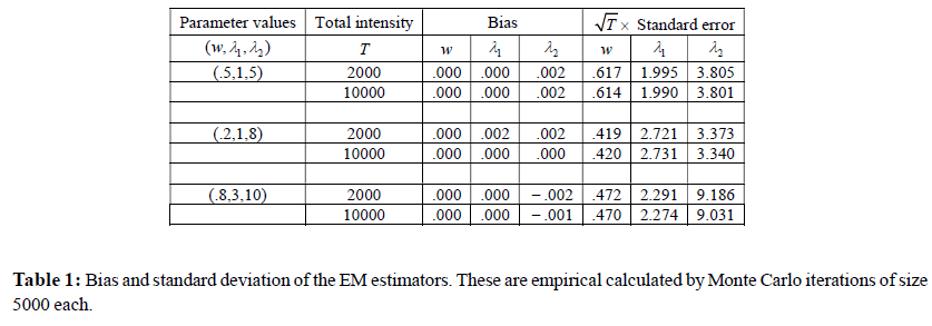
A simulation study is presented for evaluating the bias and standard deviation for the estimated parameters for two different total intensity sizes T = 2,000 and 10,000 respectively. As before, T denotes the sum of the intensities of the clusters of successive features and thus these choices of T are realistic. For each T , the distribution of the data is chosen to be a locationshifted mixtures of Poisson, with mixing parameters w and the mean parameters λ₁ and λ₂, respectively. This means that approximately w × 100% of the data are generated from Poisson distribution with parameter λ₁ and the remaining (1-w)×100% of the data are generated from Poisson distribution with parameter λ₂ + 1. We report the results for three sets of values of these parameters. For each of the data set generated from the mixture distribution, the maximum likelihood estimates are obtained for the three parameters, w, λ₁, and λ₂, via the EM algorithm described in Section 2. The estimates of the bias and standard deviation are obtained by 5,000, Monte Carlo iterates for each setting.

Empirical Sizes of the Proposed Tests

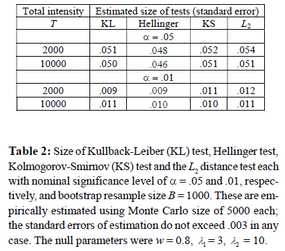
In the second simulation, the empirical sizes of the four tests (the KL test, the Hellinger test, the KS test and the L2 distance test) are investigated. The data is generated using the same scheme as in Simulation 1. For the sake of brevity, we only report the results (Table 3) the values for w = 0.5, λ₁ = 1, λ₂ =5. We compute the sizes of the tests by the empirical proportions of times the null hypotheses are rejected by each of these tests in 5,000Monte Carlo samples for each total intensity size.

Empirical Powers of the Proposed Tests

In order to study the effectiveness of our method, a power analysis is conducted. It can be seen from the second simulation (see, Section 3.4 or Table 3), all four tests maintained the prescribed significance level. As a result, all of them are included in our power study. The power of each of the four tests is evaluated at two types of alternative hypothesis models by Monte Carlo Simulation.

In the first alternative, we study the empirical power when there are additional gross errors in the two-component location- shifted mixture of Poisson model. More precisely, the data are generated from a contaminated distribution given below:

(1 - δ)F₁ + δF₂, 0 ≤ δ ≤ 1, (6)

where F₁ is the null model of a two-component locationshifted mixture of Poisson and F₂ is a uniform distribution on the set of integers between 0 and 4. In effect, part of the data came from the F₁ and the rest of the data were generated from the contaminating uniform distribution. Note that under no contamination, i.e., δ = 0 , one recovers the null model. We vary the contamination factor δ in [0,1].

In the second alternative, the data are generated from a discretized (rounded) version of a normal distribution, which is supported on integers {0,…K} with probabilities proportional to

for x = 0,1,…,K . Here λ is a parameter of the distribution and K is a large enough integer such that p_x < 10^-4 for x > k.

Results for the Simulation Study

Consistent convergence (statistical consistency) to the true values with increasing total intensity is seen in Simulation 1. The results are illustrated in Table 1. For all the parameters: w, λ₁, λ₂ the bias decreases as total intensity increases. In order to investigate the asymptotic ( as T —> ∞ ) standard deviation, we report the empirical standard deviations multiplied by the square root of the total intensity T and in all cases they seem to be stabilized.

In Simulation 2, the empirical sizes of the four tests are investigated. Table 2 shows the empirical sizes for the four tests, given the Monte Carlo size of 5,000, the number of bootstrap samples B = 1,000 and the commonly used nominal significance levels of α = 0.05 and 0.01, respectively Convergence to the nominal sizes with increasing total intensity is observed in these simulations for all the tests. Overall, the size of all the tests remains approximately equal to the α.

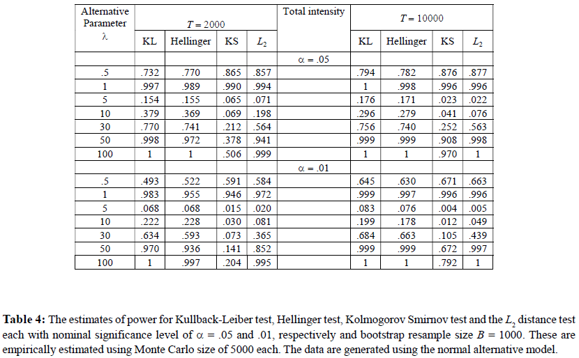
As stated before, in the third simulation, we study and compare the empirical powers of the above tests against the two alternative hypotheses. We used the same values of T , B, Monte Carlo size and the nominal level α as in Simulation 2. The results for the first and the second alternative hypotheses are reported in Table 3 and Table 4, respectively.

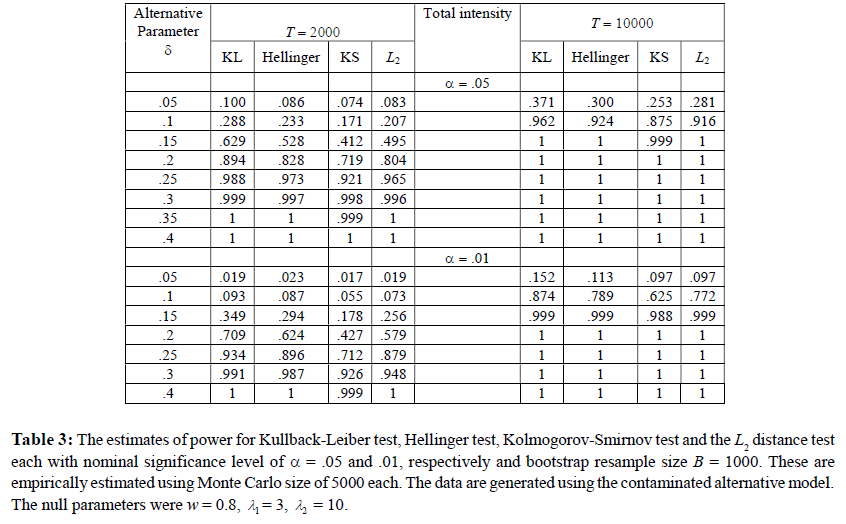
For the first alternative the data is generated following model (6). We investigate the powers for a set of null parameter values w=0.8, λ₁ = 3, λ₂ = 10 for the locationshifted Poisson distribution. The contaminating distribution is discrete uniform on the set of integers from 0 to 4 and a range of contaminating weight factor δ (=.05 to .4). The results are reported in Table 3. The power function of all the tests increase monotonically in δ (as the alternative moves further and further away from the null hypothesis) reaching one in all cases for forty percent contamination. Furthermore, the power curve for T = 10000 lies above the power curve for T = 2000 which is to be expected from the theory. The power of the KL test appears to be the largest in all cases making it the recommended choice. The Hellinger tests comes in a close second.

For the second alternative, Table 4 shows the result of the empirical power of the same four tests against different values of the alternative model parameter λ ( = 0.5, 1, 5, 10, 30, 50, 100). Unlike the previous scenario, the null hypothesis is not embedded in H₀ and λ does not measure a distance’ from the null. As a result, the power function show a non-monotonic pattern which eventually becomes monotonic for large λ. Once again, the KL and the Hellinger tests take the first two places and display very decent power in most cases. Once again, the power of each test increases with the total intensity T.

Based on these simulation results, we use the KL test for data analysis to be described in the next section.

We consider a previously published data of human plasma samples (Mantini et al., 2007) collected from thirty healthy human subjects (age 28-40 years) for the demonstration of our peak detection method. The original unprocessed data, as expected, was contaminated by baseline drifts and background noises. The plasma data was baseline corrected using the bslnoff function (with method = loess and bw = .025) in PROcess package mentioned earlier. A schematic overview of detecting monoisotopic peaks in each sample is given in Figure 1.

Figure 1: Schematic representation for monoisotopic peak detection.

Summary of Peak Detection Results

In order to avoid degeneracy in the parameter estimation process and for greater biological reliability we only consider clusters of features each with at least four members. From the results discussed in the previous section the KL test appears to be the most superior in the simulation studies, and hence it is used to test and identify the monoisotopic peaks of a MALDITOF data from plasma samples. Below, we report the identified monoisotopic peaks for the samples and compare the performance of our method with another peak detection method due to Mantini et al., (2007). For brevity of presentation, we report the results of five selected spectra. The conclusions are similar for other spectra and can be found on the supplementary web-site (www.susmitadatta.org/Supp/MP ).

Since the noise threshold in the denoising step of the preprocessing of spectra is user selectable, we perform a sensitivity analysis of our results by selecting different threshold values Table 5 shows the number of monoisotopic peaks detected on each sample or subject for different denoising cutoff. For example, the number of monoisotopic peaks detected in Spectrum 1 are 18, 13 and 13 for thresholds h = 100, 150 and 200, respectively. The sixth and the seventh column of Table 5 report the common monoisotopic peaks within each sample for varied denoising cutoff h. For example, there are eleven detected monoisotopic peaks in Spectrum 1 that are in common when applying our procedure with h = 100 and h = 150. On the other hand, there are eight common monoisotopic peaks between noise thresholds of 100, 150 and 200 in Spectrum 1. Overall, there is decent amount of overlaps (at least 60%) between the results run at thresholds of 150 and 200. This percentage is considerably lower between h = 100 versus 150 or 200. Based on this sensitivity analysis, we would recommend using h = 200 for this dataset.

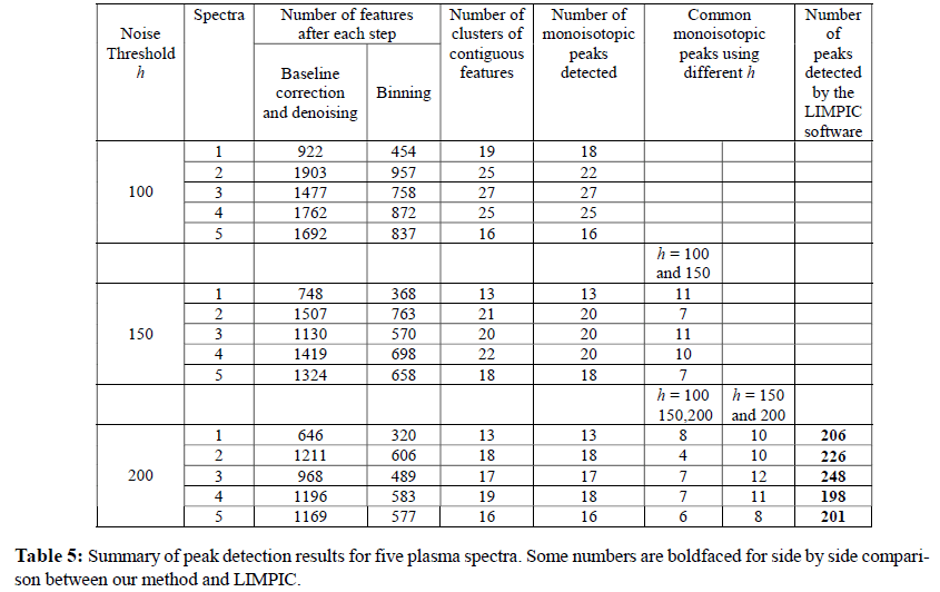
We also keep track the number of features at each step and we report the number of them when the initial preprocessing and the binning are done. For example, the number of features in subject after preprocessing is (2nd column, Table 5) and 454 after binning (3rd column, Table 5). Number of candidate isotopic distributions in each spectrum is reported in the 4th column.

Biochemical Validation

We compare the list of monoisotopic peaks detected by our method with the theoretical peptides generated by in sillico digestion of the 69 human plasma proteins mentioned in Mantini et al., 2007 (http://www.biomedcentral.com/content/supplementary/1471-2105-8-101-s5.pdf). These have been chosen by them as they can be obtained from the Human Plasma Proteome database (HPPP) (Omen et al., 2005) and can be detected on a MALDI-TOF platform in the m/z range of 5-20 kDa (Hortin, 2006). For the initial characterization of the peptide fragments, we have used in sillico trypsin digestion to obtain the peptide fragments of the candidate proteins. We have used “PeptideMass” tool (http://ca.expasy.org/tools/peptide-mass-ref.html) by Wilkins et al., (1997) and Gasteiger et al., (2005) for this purpose. For the search, we included only masses of unmodified cysteines. We have allowed peptide fragments off masses greater than 1500 Da, maximum number of five missed cleavages and included all post-translational modifications.

We consider all the peptide fragments of all these proteins and match them with the detected monoisotopic peaks only from the five samples individually. As we have binned the data only to represent the integers associated with the m/z values we round all the theoretical masses obtained from the in sillico digestion as well. We also use the accuracy level of up to 0.5. The percent of true matched peaks from each of the five samples amongst the monoisotopic peaks selected by our algorithms are 60%, 50%, 53%, 55% and 56%, respectively, for the five spectra reported earlier. Note that the data is collected from a linear MALDI-TOF instrument and the sensitivity of such platforms are generally low. Also, sample preparation did not involve immunoaffinity based methods to control the interference of highly abundant proteins like albumin. Considering all that, the performance of our method seems to be quite satisfactory.

Comparisons with Other Methods

We compare the number and the quality of the detected peaks by our method with that using the LIMPIC software developed by Mantini et al., (2007). As expected, our method detected a much fewer number of peaks compared to LIMPIC Table 5, rightmost column). This is presumably due to the fact that we detect only the monoisotopic peak amongst all the peaks in a isotopic distribution and the other procedure detects more local peaks. Figure 2 demonstrates this phenomena clearly where we show four isotopic distributions (taken from different samples). In each case, there are several features (solid lines) declared as “peaks” by LIMPIC and only one monoisotopic peak (denoted by a carat symbol on the horizontal axis). Note that in each case, the monoisotopic peaks detected by our method attain the maximum intensities on each extracted isotopic distribution.

Figure 2: An illustration of the comparative nature of the two peak detection . algorithms as applied to four clusters of contiguous features of multiple spectra. A smoothed version of the intensity values is displayed. The location of the (monoisotopic) peak detected by our method is indicated by a carat and a solid vertical line; the locations of the multiple peaks detected by the LIMPIC software are denoted by dashed vertical lines.

We have also attempted to apply a proprietary software implementation of (Breen et al., 2000, 2003 ). However, their procedure is integrated with the entire preprocessing routine which requires the user to specify a number of parameters. In addition, the software requires specification of various types of MALDI preparation all of which are not available for this dataset. We have made several abortive attempts to detect peaks using their software for this dataset by selecting various combinations of parameters.

It is natural to believe that more intense peaks are more sensitive for a biomarker study. Identification of chemically valid lesser number of peaks is less prone to the difficulty arises with analysis of large number of variables and a much lower sample sizes without loosing important information. Also, lesser numbers of intense peaks are suitable to classify samples using much simpler classification algorithms like LDA or QDA. We plan to pursue the comparative study in a classification context in a follow-up paper.

Peak detection in a mass spectra is an important step in applying proteomic profiling to biomedical research. As for example, the detected peaks can be subsequently investigated in discovering relevant biomarkers. Also it serves as a feature reduction tool so that further statistical and data analytic techniques can be used on a sample of mass spectra. In addition, it separates true signals from the background noise. This is imperative since a mass spectrum is inherently noisy.

While most attempts in the past concentrates on separating large signals (after baseline correction and sometimes after local standardization) from small intensity noise background, this does not, in general, guarantee the quality of the detected peaks. Not all large signals are biodoes not, in general, guarantee the quality of the detected peaks. Not all large signals are biochemically viable; in addition, in or around a true monoisotopic peak, there may be other large secondary signals. Thus, care needs to be taken in order to identify only the monoisotopic peaks in a spectrum. On one hand, this ensures maximum filtration and data reduction. On the other hand, the resulting channels (features) are likely to provide higher specificity in a case-control or classification study. We are planning to investigate this with our peak detection technique in a future manuscript.

We present a novel approach for detecting the monoisotopic peaks, where we considered fitting a class of mixture location-shifted Poisson models with two components. Unlike previous attempts, our procedure is local and automatic in the sense that it works with each individual spectrum without requiring detailed information regarding specific settings of the spectrometer, the matrix elements and so on. We utilize statistical methods rather than database information in estimating parameter in the model. In addition a call is made using formal statistical tests with a specified type 1 error rate rather than ad hoc cutoffs.

As demonstrated with simulated and real data, the methodology the presented here is implementable and produces reasonable answers in a wide variety of settings. In addition, only high quality peaks are detected in a spectrum which might improve mass spectrometry based classification error rate of normal versus diseased samples. We plan to explore this elsewhere.

Our monoisotopic peak detection method identifies a much smaller number of peaks (compared to other peak detection methods) which are unique peaks in isotopic clusters of peptide molecules. These monoisotopic peaks are expected to perform much better in terms of classification accuracy in a case control study. As a preliminary observation we have attempted to classify mouse amniotic fluid data (Datta et al., 2008) for a case control study with the monoisotopic peaks determined from our method and also by LIMPIC (Mantini et al., 2007). The area under the ROC (Receptor Operating Curve) for our peaks were much greater and also the overall classification accuracy (results not shown) while using these features in a SVM (support vector machine). However, it is to be noted that the classification performance depends on particular classification algorithms, the tuning parameters and also cross validation procedures. Therefore, we are currently working on an exhaustive study on the comparative classification performances and we will report the results elsewhere.

This work is supported by the grant NSF DMS- 0805559 awarded to Susmita Datta. We also wanted to thank Dr. Somnath Datta for his helpful comments.