Journal of Defense Management
Open Access
ISSN: 2167-0374
ISSN: 2167-0374
Review Article - (2016) Volume 6, Issue 2
In 2003, LTC Cantwell proposed a methodology using zero-sum games to improve military decision making in choosing courses of action. He proposed using ordinal values to fill in the zero-sum payoff matrix for the USA and the opponent and then solve the game. We propose a method and illustrate his example after we have replaced the ordinal values with cardinal values using multi-attribute decision making techniques. The result should be more meaningful with more accurate preferences and utilities. We extend the analysis by transforming the game from a zero-sum to a non-zero sum game and examined the solutions. Comparisons are made and discussed.
Keywords: Two person zero-sum game; Two person non-zero sum game; Game theory; Military decision process; Multi-attribute decision making; Analytical hierarchy process
In 1950, Haywood proposed the use of game theory for military decision making while at the Air War College. This work culminated in an article, ‘Military Decisions and Game Theory” [1]. Further work by Cantwell [2] showed and presented a ten step by step procedure to assist analysts in comparing courses of action for military decisions. He illustrated his method using the Battle at Tannenberg between Russia and Germany in 1914 as his example [3].
Cantwell’s ten step procedure [2] was presented as follows:
Step 1: Select the best-case friendly course of action for the friendly forces that achieves a decisive victory.
Step 2: Rank order all the friendly courses of action from best effects possible to worse effects possible.
Step 3: Rank order the enemy courses of action from best to worst in each row for the friendly player.
Step 4: Determine if the effect of the enemy courses of action result in a potential loss, tie or win for the friendly player in every combination across each row.
Step 5: Place the product of the number of rows multiplier by the number pf column in the box representing the best case scenario for each player.
Step 6-9: Rank order all combination for wins, tie, and loses descending down from the value of Step 5 to 1.
Step 10: Put the matrix into a conventional format as a payoff matrix for the friendly player.
Now, the payoff matrix is displayed in Table 1 after executing all 10 steps. We can solve the payoff matrix for the Nash Equilibrium. In Table 1, the saddle point method, Maximin, [4], illustrates that there is no pure strategy solution. When no pure strategy solution, exists there is a mixed strategy solution [4].
| Attack N | Attack S | Coordinatd Att |
ATT N, fix S |
Attack S, fix N | Defend in depth | Maximin | |
|---|---|---|---|---|---|---|---|
| Attack N, fix S | 24 | 23 | 22 | 3 | 15 | 2 | 2 |
| Attack S, fix n | 16 | 17 | 11 | 7 | 8 | 1 | 1 |
| Defend in place | 13 | 12 | 6 | 5 | 4 | 14 | 4 |
| Defend along Vis | 21 | 20 | 19 | 10 | 9 | 18 | 9 |
| Minimax | 24 | 23 | 22 | 10 | 15 | 18 | No saddle |
Table 1: Cantwell’s payoff matrix.
Using linear programming [4-7] the game is solved obtaining the following results:
V=9.462 when “friendly” chooses x1=7.7%, x2=0, x3=0, x4=92.3% while “enemy” best results come when y1=0, y2=0, y3=0, y4=46.2% and y5=53.8%.
The interpretation, in military terms, appears to be that player one should feint an attack north and fix south while concentrating his maximum effort to defend along the Vistula River or they can leak misinformation slightly about the attack and maintain secrecy. Player two could mix their strategy: attack north-fix south or attack south- fix north. The value of the game, 9.462 is a relative value that has no real interpretation [2]. According to Cantwell the results are fairly accurate as to the decisions.
We propose a methodology change to obtain more representative preferences using multi attribute decision making, specifically AHP’s pairwise comparison method. The reason we make this recommend is that ordinal numbers should not be used with mixed strategies. For example if player A wins a race and player 2 finishes second, what does it mean to subtract the places? It makes more sense to have collected the times of the race and then subtract where the differences have real meaning and interpretation.
Mixed strategies methods results in probabilities to play strategies that must be calculated utilizing mathematical principles. You cannot add, subtract, multiply, or divide ordinal numbers and make sense of the results.
AHP and AHP-TOPSIS hybrids have been used to rank order alternatives among numerous criteria in many areas of research in business industry, and government [8] including such areas as social networks [9,10], dark networks [11], terrorist phase planning [12,13] and terrorist targeting [14].
The following table represents the process to obtain the criteria weights using the Analytic Hierarchy Process used to determine how to weight each criterion for the TOPSIS analysis. Using Saaty’s 9 point reference scale [15], displayed in Table 2, we used subjective judgment to weight each criterion against all other criterion lower in importance. Figure 1 displays the template used.
| Intensity of Importance in Pair-wise Comparisons | Definition |
|---|---|
| 1 | Equal Importance |
| 3 | Moderate Importance |
| 5 | Strong Importance |
| 7 | Very Strong Importance |
| 9 | Extreme Importance |
| 2,4,6,8 | For comparing between the above |
| Reciprocals of above | In comparison of elements i and jif i is 3 compared to j,then j is 1/3 compared to i. |
| Rationale | Force consistency; measure values available |
Table 2: Saaty’s 9-point scale.

Figure 1: AHP Template.
We begin with a simple example to illustrate. Assume we have a zero-sum game where we might know preferences in an ordinal scale only.
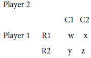
Player 1’s preference ordering is x>y>w>z. Now we might just pick values that meet that ordering scheme, such as 10>8>6>4 yielding
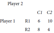
There is no saddle point solution to this game. To find the mixed strategies, we could use the method of oddments. The method of oddment finds Player I plays R1 and R2 with probabilities ½ each and Player II plays ¾ C1 and ¼ C2. The value of the game is 7.
The probabilities are function of the values chosen in the payoff matrix and not reflective of the utility the player has for each set of strategies.
Therefore, rather than arbitrary values or even using the lottery method of von Neumann and Morgenstern [5] we recommend using AHP to obtain the utility values of the strategies.
We begin by numerating the strategies combinations in a subject priority order R1C2>R2C1>R1C1>R2C2. Then we use the pairwise values from Saaty’s 9 point scale in Table 2 to determine the relative utility. We prepared an Excel template to assist us in obtaining these utility values, as shown in Figure 1. In this template the prioritized strategies are listed so we can easily perform pairwise comparisons of the strategies.
We obtained the following AHP pairwise comparison matrix as shown in the Table 3.
| x | w | y | z | ||
|---|---|---|---|---|---|
| 1 | 2 | 3 | 4 | ||
| 1 | x | 1 | 3 | 5 | 7 |
| 2 | w | 01-Mar | 1 | 2 | 4 |
| 3 | y | 01-May | 01-Feb | 1 | 3 |
| 4 | z | 01-Jul | 01-Apr | 01-Mar | 1 |
Table 3: AHP pairwise comparison matrix.
The consistency ratio of this matrix, according to Saaty’s work [15], must be less than 0.1. The consistency of this matrix was 0.0021, which is smaller than 0.1. We provide the formula and definition of terms.
The Consistency Index for a matrix is calculated from (λmax-n) /(n- 1) and, since n=4 for this matrix, the CI is 0.00019. The final step is to calculate the Consistency Ratio for this set of judgements using the CI for the corresponding value from large samples of matrices of purely random judgments using the Table 4, derived from Saaty’s book, in which the upper row is the order of the random matrix, and the lower is the corresponding index of consistency for random judgements. CR=CI/RI
|
N |
1 |
2 |
3 |
4 |
5 |
6 |
7 |
8 |
9 |
10 |
11 |
12 |
13 |
14 |
15 |
|
RI |
0 |
0 |
0.58 |
0.9 |
1.12 |
1.24 |
1.32 |
1.41 |
1.45 |
1.49 |
1.51 |
1.48 |
1.56 |
1.57 |
1.59 |
Table 4: Samples of matrices of purely random judgments.
For this example, that gives 0.00190/0.90=0.0021. Saaty argues that a CR<0.1 indicates that the judgements are consistent.
We obtain the weights, which are the eigenvector to the largest eigenvalue. They are presented here to three decimals accuracy.
x=0.595
w=0.211
y=0.122
z=0.071
Thus, AHP can help obtain the relative utility values of the outcomes. These values are the cardinal utilities values based upon the preferences. The game with cardinal utilities is now
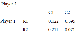
If we apply oddment to this game, we find Player I plays 22.8% of the time R1 and 77.2% of the time R2 while Play II plays C1 85.5% of the time and C2 14.5% of the time. The value for the revised game based on cardinal utility is 0.190.
Proposed application of AHP to the military decision making example
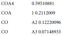
Two person zero-sum game: The row player has four courses of action that might be compared initially. We provide an initial preference priority COA 4, COA 1, COA 2, COA 3 shown in Figure 2.

Figure 2: COA1-COA 4 Weighting analysis.
The consistency ratio is 0.002 which is less than 0.10 [15]. The weights calculated by the AHP template [16] are:
Now under each we will obtain weights as functions of the enemy COAs. For example, we display Figure 3.

Figure 3: Enemies ECOA1-ECOA6 under player 1’s COA1.
The consistency ration is CR=0.03969 (less than 0.1 is acceptable). We find the sub weights from the template.
The sub-weights are
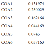
To obtain the useable weights we form the product of COA 1 times these sub weight values.
0.091146
0.052756
0.034217
0.00932
0.01572
0.007841
We repeat the process for friendly COA 2 through friendly COA 4 for the enemies COA-1COA 6 displayed in Table 5.
| Major Criteria-Row Player | Local Weights | Sub Criteria | Local Weights | Global Decision Weights (Criteria Weight x Sub Criteria Weight) |
|---|---|---|---|---|
| Player 2 | ||||
| COA 4 | 0.595 | COA 1 | 0.431974 | 0.091146 |
| COA 2 | 0.25 | 0.052756 | ||
| COA 3 | 0.162 | 0.034217 | ||
| COA 4 | 0.404 | 0.00932 | ||
| COA 5 | 0.0745 | 0.01572 | ||
| COA 6 | 0.0372 | 0.007841 | ||
| COA 1 | 0.211 | COA 1 | 0.033223 | |
| COA 2 | 0.054067 | |||
| COA 3 | 0.016419 | |||
| COA 4 | 0.006478 | |||
| COA 5 | 0.007619 | |||
| COA 6 | 0.004395 | |||
| COA 2 | 0.122 | COA 1 | 0.017705 | |
| COA 2 | 0.013371 | |||
| COA 3 | 0.005412 | |||
| COA 4 | 0.004151 | |||
| COA 5 | 0.003779 | |||
| COA 6 | 0.027081 | |||
| COA 3 | 0.0715 | COA 1 | 0.235044 | |
| COA 2 | 0.134041 | |||
| COA 3 | 0.079026 | |||
| COA 4 | 0.037179 | |||
| COA 5 | 0.030092 | |||
| COA 6 | 0.079718 |
Note that the SUM of all weights=1
Table 5: Obtaining the payoff.
These 24 entries are now the actual entries in the game matrix corresponding to R1-R4 for player 1 and C1-C6 for player 2 in this combat analysis.
We developed a template to solve, via linear programming larger zero sum games such as this game [7].
Based upon these preference values, we enter our linear programming model template for game theory, displayed in Figure 4.

Figure 4: Results using cardinal values in the combat analysis payoff matrix.
The results show a pure strategy solution that indicated Player 1 should defend the Vistula River and Player 2 should attack south, fix north to obtain their best outcomes. This is consistent with Cantwell’s results but perhaps more accurate since the values are based upon preferences not just ordinal rankings from 24 to 1.
Sensitivity analysis: We used Equation (1) [17] for adjusting weights of the primary COAs for player 1 and obtain new weights for the payoff matrix.
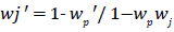 (1)
(1)
Where wj’ is the new weight and wp is the original weight of the criterion to be adjusted and wp’ is the value after the criterion was adjusted. We found this to be an easy method to adjust weights to reenter back into our model.
We summarize some of the results in Table 6 that includes only the strategies for each player.
| Strategy Played | Ordinal Preferences Cantwell | Cardinal Preferences | Sensitivity #1 | Sensitivity #2 | Sensitivity #3 |
|---|---|---|---|---|---|
| Player 1 | |||||
| COA 1 | 0.077 | 0 | 0.28 | 0.25 | 0 |
| COA 2 | 0 | 0 | 0 | 0 | 0 |
| COA 3 | 0 | 0 | 0 | 0 | 0 |
| COA 4 | 0.923 | 1 | 0.72 | 0.75 | 1 |
| Player 2 | |||||
| COA 1 | 0 | 0 | 0 | 0 | 0 |
| COA 2 | 0 | 0 | 0 | 0 | 0 |
| COA 3 | 0 | 0 | 0 | 0 | 0 |
| COA 4 | 0.462 | 0 | 0.567 | 0.77 | 0 |
| COA 5 | 0.538 | 1 | 0.433 | 0.23 | 1 |
| COA 6 | 0 | 0 | 0 | 0 | 0 |
Table 6: Game and analysis summary.
We find the splayer 1 should always play strategy 4 either 100% or over 70%. Clearly that indicates a favourable strategy. If player 2 plays either a pure strategy with their COA 5 or a mixed strategy of COA 4 and COA 5 as indicated in the Table 6 to minimize their loss.
There is no reason to assume that the game must be a zero sum game. Cantwell’s method can be employed for the player 2 side to construct payoff that are in fact non-zero. Additionally we might use the AHP method as we did to obtain player 1 values for player 2. We used the nonlinear programming approach presented in Barron [18].
Nonlinear Programming Approach for two or more strategies for each player
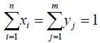
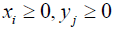
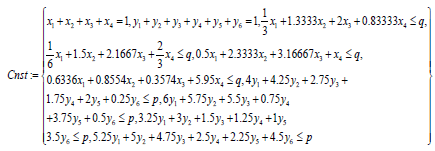
For games with two players and more than two strategies each, we present the nonlinear optimization approach by Barron [18]. Consider a two person game with a payoff matrix as before. Let’s separate the payoff matrix into two matrices M and N for players I and II. We solve the following nonlinear optimization formulation in expanded form, in equation (1).
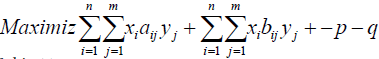 Subject to
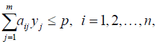
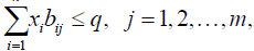 (2)
(2)
We developed a Maple routine from Barron [18] to perform our calculations.
With (Linear Algebra): With (Optimization):
A:= Matrix([[6,5.75,5.5,0.75,3.75,0.5],[4, 4.25, 2.75,1.75, 2,0.25], [3.25,3,1.5,1.25,1,3.5],[5.25,5, 4.75, 2.5, 2.25, 4.5]);]
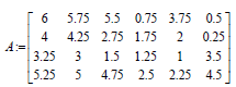
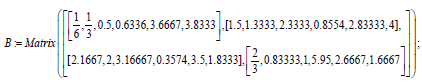


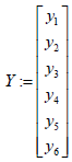


objective := exp and(Transpose(X ).A.Y +Transpose(X ).B.Y − p − q);

The NLP solution found was that Player 1 plays COA 4 and player 2 plays COA 4.
NLPSolve(objective,Cnst,assume = nonnegative,max imize,initialpoint = {p = 3,q = 6})
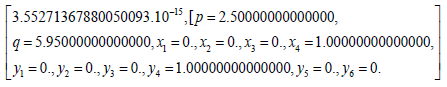
The key result here is that after we analyzed this game as a non-zero game, player 1’s choice was still COA 4.
Although we presented methodologies to more accurately depict the use of game theory be using cardinal utilities, we only illustrated with the Tannenberg example from Cantwell. However, the results are promising enough to continue to employ these methodologies to assist military planners and decision makers, Game theory does provide insights in how to play a game and therefore, we conclude that it does provide insights into military planning and strategy.