Journal of Aeronautics & Aerospace Engineering
Open Access
ISSN: 2168-9792
ISSN: 2168-9792
Research Article - (2016) Volume 5, Issue 2
We computed magnetic field gradients at satellite altitude, over Europe with emphasis on the Kursk Magnetic Anomaly (KMA). They were calculated using the CHAMP satellite total magnetic anomalies. Our computations were done to determine how the magnetic field observations data from the new ESA/Swarm satellites could be utilized to determine the structure of the magnetization of the Earth’s crust, especially in the region of the KMA. Ten years of CHAMP data were used to simulate the Swarm data. An initial east magnetic anomaly gradient map of Europe was computed and subsequently the North, East and Vertical magnetic gradients for the KMA region were calculated. The vertical gradient of the KMA was also determined using Hilbert transforms. Inversion of the total KMA was derived using Simplex and Simulated Annealing algorithms. The depths of the upper and lower boundaries are calculated downward from the 324 km elevation of the satellite. Our resulting inversion depth model is a horizontal quadrangle. The maximum errors are determined by the model parameter errors.
<Keywords: Earth's magnetic field; Gradients
The gradients of total magnetic field anomalies over regions of Europe and Kursk can be regarded as some previous computations before processing and interpretation of the measurements of the SWARM satellites. They are launched at November 22, 2013. The gradients of the total magnetic anomalies can be directly determined by the measurements of the SWARM satellites. But the gradients can be determined by appropriate procedures of the earlier satellites e.g. the CHAMP satellite operated between July 15, 2000 and September 19, 2010. Inversion of the magnetic anomalies horizontal and vertical gradients can provide details on the source region.
The exploitation of iron deposits has a great economic importance. The Kursk Magnetic Anomaly is located 400 km south of Moscow it is one of the largest magnetic anomaly on Earth. The Proterozoic iron ore deposits are located in a NNW-SSE oriented complex syncline which is superimposed on the Voronezh Bulge anteclise. The Voronezh Bulge is bordered by the Ryazan-Saratov and Pripyat-Dnieper-Donetsk aulacogens Shchipansky and Bogdanova [1]. The extent of the anomaly is approximately 190,000 km2 and its crustal depth is between 0.5 - 3.0 km. According to Heiland [2] the anomaly was discovered by Smirnov in 1874. The discussion of the anomaly is described by the early works of Lasareff [3], Haalck [4] and more recent investigations by Lapina [5], Taylor and Frawley [6], and Rotanova [7]. Due to its extent and large magnetization it can be detected by satellite measurements (Magsat, Taylor and Frawley 1987; The resultant magnetization is 3 Am-1 (Taylor and Frawley [6]. Our inversion computations are based on their value. The direction of the resultant magnetization is 47° East declination 67° down inclination. The Kursk magnetic anomaly was computed 324 km altitude from CHAMP measurements Figure 1 Kis et al. [8].

Figure 1: Kursk total magnetic anomaly map computed from CHAMP satellite data at 324 km altitude and plotted in an Albers Equal area conic projection. C. I.=2 nT.
The texture of iron ore bodies can be banded iron formation (BIF) and/o granular iron formation (BIF), Bekker et al. [9]. These marine sediments were formed in the Archean and Paleoproterozoic. Their maximum age is 2.6 ca. Ga. The BIF were dominant in the Archean and earliest Paleoproterozoic while GIF were in the later Paleoproterozoic. A summary of these geological processes which formed the Kursk iron-ore structures are given in Voskresenskaya [10], Alexandrov [11], Shchipansky and Bogdanova [1], Bekker et al. [9], Kovács and Pálfy [12].
These deposits contain considerable qualities of iron in siliceous banded structures. One theory is that the iron originated from marine and submarine volcanic activities or the possible from mantle plumes near the sea bottom. The precipitation of iron depends on the redox conditions of the environment, since the reduced Fe (II) remains as a liquid while the oxide Fe (III) precipitates in anoxic setting. The formation of iron deposits was prevented by the Great Oxidation Event ca. 2.4 Ga. The reductive environment of the hydrosphere ended and the oxygen content increased. This event was due to the decline of volcanic activities. The production of BIF’s may have reached a maximum at ca 1.85 Ga, since the magmatic activity was greater at this time. The composition of BIFs and GIFs indicates that it is probably of submarine origin.
Three possible oxidative processes are summarized by Bekker et al. [9]. The first description: the origin of the oxygen is from a photosynthetic process of cyanobacteria in the a thin oxidative zone in the upper layer of the sea.. Under this layer there are some anoxic water columns where Fe (III) precipitates. According to the second version the iron oxidizing bacteria live in an anoxic environment. These proto-bacteria are able to absorb water and carbon dioxide. The third process: ultraviolet photons oxidize the Fe (II) liquid to Fe (III) solids. Bekker et al. [9] state that the third process is less probable.
The gradients of the magnetic field can be determined directly from the from the two side by side lower orbiting SWARM satellites. The gradients of the magnetic field can also be computed from the CHAMP anomalies.
Previously we Taylor et al. [13] calculated the horizontal gradients over the Kursk magnetic anomaly. In this study the vertical, north and east gradients will be computed.
CHAMP magnetic anomalies over the European region and the KMA were calculated at 324 km altitude. These anomalies are plotted in a spherical polar coordinate system Kis et al. [8] (Figure 2).

Figure 2: Total magnetic anomaly map over part of Europe at 324 km. C. I.= 2nT.
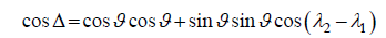
The anomaly data in Figure 2 are at the same latitude but different longitude. The spherical distance Δ between two data values is given by the spherical triangle cosine theorem:
 (1)
(1)
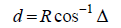
Where  is the polar distance, λ2 and λ1 are the two longitudes, respectively. The distance of these two data is given by given by the equation:
 (2)
(2)
Where R is the Earth’s spherical radius, 6371.2 km + 324 km. The Eastern gradients are approximated by the simple equation of
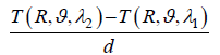 (3)
(3)
where T indicates the total magnetic anomaly. The East gradients determined by this method are shown in Figs. 3, 4 and 5. The longitude distance, λ2-λ1 was 1° the East gradients are shown in Figure 3. In this case the d distance varies between 88.86 and 49.75 km due to the meridional convergence. The longitudinal distance is 2° in Figure 4, and distance d is between 177.71 and 99.51 km, while the distance d is changed between 355.42 and 199.02 km. It can be seen from Figures 3-5 that the appropriate spherical distances will be 1° or 2° for the gradient determination for the SWARM anomalies.

Figure 3: East gradient contour interval is 0.2 nT/km spherical distance is 1 degree.

Figure 4: East gradient of European total magnetic anomalies (figure 2) at 324 km altitude (Albers projection) Spherical distance is 2 degrees.

Figure 5: East Gradient of European total magnetic anomalies (Figure 2) spherical distance is 4 degrees.
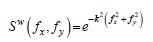
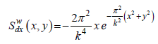
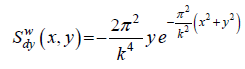
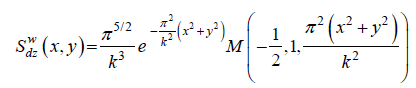
The second method for computing the gradients is based on the application of the transfer and weight functions of the x-, y- and z- axes Kis and Puszta, [14]. The transfer functions of the above mentioned gradients are given by Blakely [15]:
 (4)
(4)
Where Sdx, Sdy and Sdz are the transfer functions of the x-, y- and z- gradients; fx and fy are the spatial frequencies, j is the imaginary unit. Gaussian low-pass window of:
 (5)
(5)
Is applied for the above mentioned transfer functions, where k is the appropriate parameter of the windowed transfer functions. The weight functions of the windowed transfer functions are:
 (6)
(6)  (7)
(7)  (8)
(8)
Where M is the confluent hypergeometric function (Slater, 1976). The development of the (6) – (8) functions is given by Kis and Puszta [14].
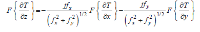
If the gradients are computed by the above method than the CHAMP anomalies should be transformed from the spherical polar coordinate system to the Cartesian coordinate system. The zero of the Descartes coordinate system is placed at an altitude of 324 km and at latitude 48.75° and longitude 36.25°. The transformation is given by Kis et al. [16]. The windowed gradients are computed in the Cartesian coordinate system and next step is their transformation into the spherical polar coordinate system. These gradients are shown in the Figures 6-8 in an Albers’ projection. These gradients emphasize the depth variation or change in magnetization of the source or both. These results are not determined unambiguously from the gradients. The gradients in Fig. 6 show the Northeast- Southwest elongation of the Kursk anomalies while Fig. 7 illustrates the East-West variation. The vertical gradient, Figure 8 displays a Northwest-Southeast directional asymmetry.

Figure 6: North gradient of KMA (Fig. 1 on an Albers’ projection). C.I.=0.015nT/km.

Figure 7: East gradient of KMA (Fig. 1) in Albers’ projection. C. I.=0.015nT/km .

Figure 8: Vertical gradient of KMA (Figure 1.) C.I.=0.02 nT/km.
The third method for calculating the vertical gradient is using the Hilbert transform. The Hilbert transform was named by G. H. Hardy (1932), the English mathematician, out of deference to D. Hilbert, the German mathematician. Nabighian [17,18] Nabighian and Hansen [19] Guspi and Novara [20] applied Hilbert transforms to the analysis of potential fields.
Let us consider the equation:
 (9)
(9)
Given by Nabighian [18], where F is the Fourier transform. This equation can be expressed in a simpler form:
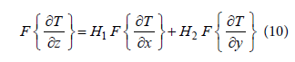 (10)
(10)
Where H1 and H2 are the Hilbert transform, that is:
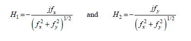 (11)
(11)
The inverse Fourier transform of Equation (9) is:
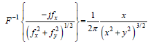 (12)
(12)
and
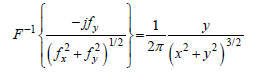 (13)
(13)
These inverse Fourier transforms are given by Nabighian [18] in his Appendix A. The CHAMP magnetic anomaly field (Fig. 1) is transformed from the spherical polar coordinate system to the Descartes coordinate system. Now the Hilbert transform is computed in the spherical polar coordinate system and the vertical gradients given in Figures 8 and 9, they illustrate virtually the same results.

Figure 9: Vertical gradient of KMA (Figure 1) computed by Hilbert transform, C.II=0.02nT/km.

Figure 10: Computed model in Cartesian coordinates data have a Gaussian distribution with the minimum problem being solved using the simplex method. The table shows the determined parameter values and their maximum error.

Figure 11: Computed model in Cartesian coordinates, the data have Gaussian distribution with the minimum problem being solved using the simulated annealing method. Table shows the calculated parameter values and their maximum error.

Figure 12: Computed model in Cartesian coordinates, , the data have a Laplace distribution with the minimum problem being solved by the simplex method. The results are given in tabular form with the determined parameter values and their maximum error.

Figure 13: Computed model in Cartesian coordinates, the data have a Laplace distribution with the minimum problem being solved by simulated annealing method. The tale in the figure show the calculated parameter values and their maximu, error.
The Bayesian inference was applied to the inversion of the Kursk Magnetic Anomaly. The Bayesian inference is widely used in the inversion procedures and is summarized by Box and Tiao [21,22], Tarantola [23], Duijndam [23,24], Menke [25], Gregory [26], Kis et al. [16] and Kis et al. [8].
The Kursk Magnetic Anomalies are shown in the spherical polar coordinate system Figure 1. The inversion procedure is applied in the Descartes coordinate system so the earlier mentioned transformation should be used. The result is given in the Descartes coordinate system that was computed from the CHAMP data.
The forward model from the inversion is a quadrangle with horizontal upper and lower levels we computed the anomaly using Plouff’s [27] method. This is an idealized model of the Kursk source [28-33]. We used 3 Am-1 average magnetization given by Taylor and Frawley [6] and the average direction of magnetization inclination 47°down and 67°East declination given by Bhattacharyya.
The basic equation of the Bayesian inference is:
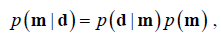 (14)
(14)
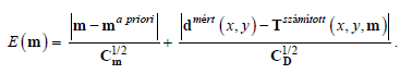
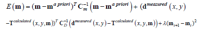
Where p (m|d) is the pa posteriori conditional probability density, p (d|m) is the likelihood conditional probability density, p(m) is the pa priori probability density. The vector m is the estimated parameters of the forward model and the vector d the measured CHAMP magnetic anomalies. The pa posteriori conditional probability density for Gaussian multivariate distribution can be expressed in the following form:
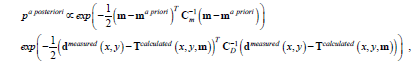 (15)
(15)
where vector ma priory is the parameters estimated by the interpreter, Cm is the covariance matrix of the estimated parameters, vector dmeasured is the measured CHAMP anomalies, Tcalculated (x,y,m) is the calculated values at the coordinate (x,y), calculated for the m parameters, CD is the covariance matrix of the CHAMP measured anomalies, superscript T the transposed vector.
The pa posteriori conditional probability density for a Laplacian distribution is:
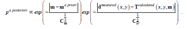 (16)
(16)
We want to maximize the pa posteriori probability density given by the equations (15) and (16) as a function of the parameter m. This is equivalent to minimizing the sum of exponent of the equations (15) and (16). The functions E (m) which will be minimized for multivariate Gaussian parameter distribution are:
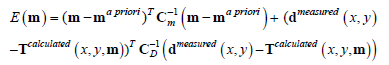 (17)
(17)
For the multivariate Laplacian parameter distribution is:
 (18)
(18)
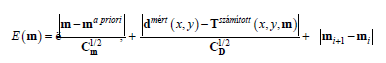
The E(m) functions equations (17) and (18) will be minimized using the regularization suggested by Tikhonov and Arsenin (1977) is:
 (19)
(19)
and
 (20)
(20)
Where λ is the regularization parameter. According to the earlier investigations Kis et al. [8] the appropriate value of λ is between 1 – 10.
The minimum problem is solved by the simplex Walsh [28] and simulated annealing Kirkpatrick et al. [29] methods. In the present investigation the a priori covariance matrix is a diagonal one whose variances is 10 km2, the likelihood covariance matrix is also diagonal one whose variances is 2 nT2. The determined models are visualized in the model values are presented in Table 1 for the Descartes coordinate system. The maximum errors are determined by the model parameter errors.
| Parameter | Gaussian distribution model parameter | Laplacian distribution model parameter | |
|---|---|---|---|
| simplex method | x1 | 500 km ± 98 km | 489 km ± 98 km |
| x2 | 438 km ± 98 km | 405 km ± 98 km | |
| x3 | -449 km ± 98 km | -379 km ± 98 km | |
| x4 | -350 km ± 98 km | -399 km ± 98 km | |
| y1 | -780 km ± 98 km | -942 km ± 98 km | |
| y2 | 399 km ± 98 km | 439 km ± 98 km | |
| y3 | 201 km ± 98 km | 321 km ± 98 km | |
| y4 | -350 km ± 98 km | -374 km ± 98 km | |
| z1 | 323 km ± 98 km | 329 km ± 98 km | |
| z2 | 331 km ± 98 km | 335 km ± 98 km | |
| simulated annealing method | x1 | 599 km ± 98 km | 650 km ± 98 km |
| x2 | 450 km ± 98 km | 449 km ± 98 km | |
| x3 | -449 km ± 98 km | -350 km ± 98 km | |
| x4 | -349 km ± 98 km | -357 km ± 98 km | |
| y1 | -650 km ± 98 km | -757 km ± 98 km | |
| y2 | 250 km ± 98 km | 350 km ± 98 km | |
| y3 | 350 km ± 98 km | 449 km ± 98 km | |
| y4 | -280 km ± 98 km | -320 km ± 98 km | |
| z1 | 309 km ± 98 km | 300 km ± 98 km | |
| z2 | 339 km ± 98 km | 339 km ± 98 km |
Table 1: Computed models in Cartesian coordinates, the data have Gaussian and Laplace distributions. The optimum problems are solved by simplex and simulated annealing methods.
The three methods for the determination of the gradients of the satellite magnetic anomaly data (at an altitude of 324 km) over the KMA are presented in spherical polar coordinates. All of them resolve the anomalies and they show the complex structure of its source. Both the windowed vertical gradient and the vertical gradient by the Hilbert transform give very similar results. All of the gradient methods can be applied. Three inversions (for Gauss distribution and the parameters determined by the simplex method; Gaussian distribution and the parameters determined by simulated annealing method; Laplacian distribution and the parameters determined by simulated annealing method) give comparable result within their maximum errors.