Journal of Stock & Forex Trading
Open Access
ISSN: 2168-9458
ISSN: 2168-9458
Research Article - (2024)Volume 11, Issue 2
With the continuous warming and cyclical fluctuations of the real estate price in China the housing price is out of balance. The method about how to make rational investment decisions has become a hot issue. Our paper aims to help people to scan properties for sale and filter out properties with the greatest potential for future appreciation so as to greatly improve the accuracy of investment decisions. This paper uses the data provided by Institute of Electrical and Electronics Engineers (IEEE) CyberC. Based on the daily data of China’s real estate prices and related influencing factors from 2012 to 2018, a mathematical model with e as the base is established for housing prices and related factors through empirical research. The ordinary least squares model with double fixed effects is used for regression model. The modeling passes the endogeneity test using instrumental variables, the heteroscedastcity test is used to verify and adjust the heteroscedastcity of the model and the Mean Absolute Deviation (MAD) test is carried out on the fit degree of the model. This paper draws the following conclusions: the model passes the significance test and there is no obvious endogenous problem. Finally the MAD test result is 0.2815.
Two-way fixed effects; OLS model; Housing price; Instrumental variable; EGLS model; Econometrics
With the rapid development of China’s economy the rising level of prices in the market has penetrated into all aspects of people’s lives and also affected people’s consumption and investment. Based on the traditional concepts of marriage and old-age care in China just in need of housing has become a hot topic. But with the rapid development of social economy people have more money to invest in commercial housing. Although the real estate industry is a link that cannot be ignored to promote the rapid development of China’s economy it also causes great fluctuations in house prices. Moreover the cyclical impact and fluctuation range brought by the real estate price fluctuation cannot be ignored. As a result the rising real estate economy and real estate prices have attracted investors from home and abroad. Therefore the current situation of the crazy rise of real estate prices and deviation from rational consumption has been formed. In order to regulate the property price, the government has introduced a series of policies to regulate the property price since 2006. The price of real estate is the result of many different but interrelated factors such as regional factors, natural environment factors, social factors, etc. As a minor in the tide of the times how to rationally purchase real estate has become a thought-provoking problem.
Theoretical background
Based on the research conducted by Cui, et al. [1] and Liang, et al. [2], a theoretical framework is built. The hedonic price theory explains that the value of housing is influenced by both the features of the property itself and the features of its surrounding area. Each feature is a combination of different housing qualities and each quality adds to the overall cost similar to a product. Homeowners and renters pay for these qualities by considering their usefulness. They are likely to balance the different qualities and the bid price shows the highest amount they are willing to pay for these qualities. Nonetheless homeowners and renters may prioritize different aspects due to their individual preferences. The revealed preference theory initially developed by economist Paul Samuelson is a technique used to study consumer choices.
It posits that consumers preferences can be understood by examining their purchasing decisions in various circumstances especially when prices vary. While we cannot directly observe the preferences of homeowners and renters in reality, “actions speak louder than words”. Hence by considering their financial limits we can infer the preferences of homeowners and renters.
Yang, et al. (2007) [3], selected 35 large and medium-sized cities in different provinces of China and conducted empirical analysis with indicators such as average house price per capita disposable income, financial participation and natural environment differential factors as the starting point. Their analysis results show that the most influential variable of real estate price is the extreme natural environment. He [4] provided theoretical support for China’s real estate research based on data analysis and econometric empirical model and discussed the factors that affect the real estate price. However in the analysis process it is only based on the unitary regression model and the data statistics are small so the empirical analysis is only a relatively simple analysis of the influencing factors of the property price.
The method proposed by Li, et al. [5], simultaneously removes fixed individual effects, selects significant variables and estimates non-zero coefficient functions. The asymptotic theory of the obtained estimation is established by selecting appropriate tuning parameters. Finally a simulation study is carried out to evaluate the performance of the proposed method and further analysis is made to illustrate the selected dataset.
Yum [6], select the panel data model with fixed effect as the standard such as Akaike Information Standard (AIC), revised Akaike Information Standard (AICc) and Bayesian Information Standard (BIC). The accompanying parameter problems may have adverse effects on short panel data. However the Monte Carlo experiment shows that the information standard is very successful in selecting real models.
Shi, et al. [7], used multiple regression analysis to analyze the real estate price in Shanghai and obtained multiple linear regression equation and tested it. Finally partial correlation coefficient analysis method and single factor weight measurement method are used to estimate the influence degree of each factor. The results show that there are obvious differences between the second-hand housing market and the new housing market. Market supply and demand are the most important factors affecting the price of second-hand housing while environmental quality is the primary factor affecting the price of new buildings.
Ye, et al. [8], evaluated and analyzed five kinds of methods for testing the mediation model, summarized the methods and processes for testing the mediation model and tested the mediation effect with the deviation corrected percentile Bootstrap method or Markov chain Monte Carlo method.
Model setting
The general model between the housing price and its influencing factors can be written as:
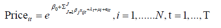
Where Priceit is the housing price per square meter in the ith city, ith time period, xj is the jth influencing factor on the housing price, λt represents a time effect that does not change with the individual at the tth time period, μi is the geographic location effect that does not change over time for the ith city, εit is the error term.
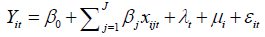
Take the logarithm of price: Y = ln (Price) also take the logarithm on the right-hand side a linear model can be derived:
Endogeneity and other problems test
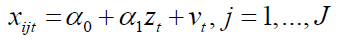
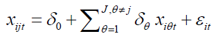
To test if there exists endogeneity problem in the model which is: E(xtεt) ≠ 0 an instrumental variable zt is set where E=(ztεt) = 0, CoV(xtzt) ≠ 0 and ztdoesn’t have direct effect on Yt. Then a 2 Stage Least Square (2SLS) regression is performed. For the first stage regression, the form is:
Then in the second stage regression, it has such a form that:
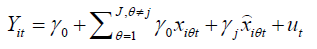
where xijt is the fitted value for xijt in step 1. If the null hypothesis H0: Yj= 0 is rejected, then it means that there exists endogeneity problem in the model.
Model validation
To test the multicollinearity problem in the model, the Variance Inflation Factor (VIF) value:
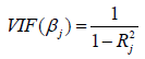
where Rj2 is the goodness-of-fit value for the regression model:
If the VIF value is higher than 10 then there exists obvious multicollinearity between xjt and the other influencing factors on the housing price.
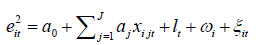
where which is the residual value in the main regression model.
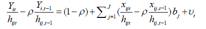
If the goodness-of-fit value R² is larger than the estimation of aj, then it can be inferred that there is heteroscedasticity problem for the jth influencing factor on housing price. If there exists heteroscedasticity problem, then an Estimated Generalized Least Squares (EGLS) transformation will be conducted on the main model which is like:

where 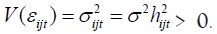 After the transformation, the auxiliary regression will be performed again on the transformed model and this step will continue until the heteroscedasticity problem totally vanishes.
After removing the heteroscedasticity problem, the autocorrelation problem will be checked, which is to say that:
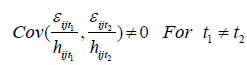
For such situation, another type of transformation will be conducted:
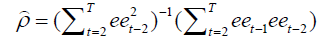
where the estimation for ρ is:
eet is the residual value in this transformed model and
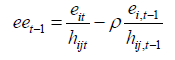
Here 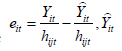 is the fitted value in the previous model with heteroscedasticity problem already removed. If R2 the goodness-of-fit value for this model is larger than the one for the previous EGLS transformed model then it can be deduced that there is autocorrelation problem for the jth influencing factor on housing price.
Data
According to the data which are provided including 34 cities from 2015 to 2018 totaling 625,968 records which are listed as below:
Data selection: First we filter and remove all lines with null values and garbled characters in the training set and test set. We use the Excel features function to convert the ‘S’ in the direction (Orient) to 1, other letters to 0 and the value of the shape ‘10’, ‘01’ to 1, the shape of ‘00’ to 0 and then filter out the value in the form of scientific notation and convert it to ordinary number form and finally rename the direction column to North-South Transparency (OrientS). We operate on the time column remove the monthly data and daily data and only retain the year. The training data in the original data contains 553098 lines and 537242 lines after cleaning. The original test set has 72870 lines and 72245 lines after cleaning (Table 1).
| Variables | Definition |
|---|---|
| Time | The date the transaction took place |
| City | The city where the transaction took place |
| District | District |
| Street | Neighbourhood |
| Community | Community |
| Lon | Longitude |
| Lat | Latitude |
| #Floors | Number of floors of the entire building |
| Floors | Approximate floor location |
| #Rooms | Number of rooms |
| #Halls | Number of halls |
| Orient | House orientation code. |
| Area | House area transaction price |
| Price | (CNY per square meter, i.e., ¥/m2) |
Note: Orient: Containing ‘N’ means the house has north facing windows; containing ‘S’ means the house has south facing windows; containing ‘E’ means the house has east facing windows; containing ‘W’ means the house has west facing windows.
Table 1: Variables and definition of North-South Transparency (OrientS).
Before conducting empirical analysis we firstly need to process the data to a certain extent.
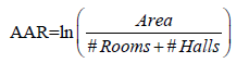
Data processing: Firstly, removing garbled and null data by filtering all data with Stata and Excel. Then setting price of the real estate as the explained variable and the Average Area per Room (AAR) as the explanatory variable, the formula is:
Besides we set the LAT (Latitude), LON (Longitude) orients as the control variables. Starting from taking the natural logarithm of latitude and longitude and then set the room orientation as a dummy variable considering the variability of room orientation. Specifically writing the south, north-south and southwest directions as 1, north, east, west, northeast, northwest and east-west orientations are set to 0. At the same time in order to eliminate the bias caused by missing variables a double fixed effect model is introduced which converts time data into annual data for time fixed effects and digitizes the city where the house is located for individual fixed effects.
Model setting
Our null hypothesis ( H0): Average areas per room, latitude, longitude, orients have influence on the house price.
According to the data cleansing, we have defined the following variables (Table 2).
| Variables | Definition |
|---|---|
| λt | Represents a time effect that does not change with the individual, |
| μi | Represents an individual geographic location effect that does not change over time, |
| i | City |
| t | Year |
| εit | Error term |
| β | Regression coefficients |
Table 2: Variables and definition of according to the data cleansing.
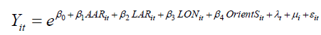
In order to test the AAR effect on the real estate price, the following double fixed-effect model is established.
Y: Take the logarithm of price, the formula is as follows:
Y = ln(Price)

Then converting the model to a linear expression the result is:
Regression results
Conducting stepwise regression on linear expressions and the result has shown (Table 3).
| Variables | 1 | 2 | 3 |
|---|---|---|---|
| Y | Y | Y | |
| AAR | -0.187150*** | -0.152147*** | -0.079674*** |
| (0.004145) | (0.003889) | (0.002383) | |
| LAT | - | -0.306101*** | 0.150464*** |
| (0.005994) | (0.00648) | ||
| LON | - | 5.655463*** | -0.646143*** |
| (0.019218) | (0.023258) | ||
| OrientS | - | -0.025627*** | -0.025365*** |
| (0.002477) | (0.001523) | ||
| _cons | 10.384023*** | - | 13.019470*** |
| - | 15.459746*** | - | |
| (0.013043) | (0.087353) | (0.109766) | |
| Year | No | No | Yes |
| City | No | No | Yes |
| N | 537242 | 537242 | 537242 |
| r2 | 0.00378 | 0.152369 | 0.693 |
| ar2 | 0.003778 | 0.152362 | 0.693562 |
Note: Standard errors in parentheses; (*): p<0.1, (**): p<0.05, (***): p<0.01.
Table 3: The main regression results along with variables.
In this model in order to study the effect of the size of the unit room on the overall real estate price, AAR is used as an explanatory variable and regressed with various other factors that may interfere with the price rate. At the same time in order to eliminate the influence of the numerical difference between variables on regression the natural logarithm is taken for the variables. To mitigate endogenous problems caused by bias in missing variables we use a fixed-effect model.
The model results show that the estimation of β1 is negative that is house prices are negatively affected by AAR and this parameter estimate result is significant at the level of 1%. The estimations of β2 and β3 are positive and negative respectively and the estimation results of each parameter are significant at the 1% level.
Endogeneity and other problems test
In this paper a double-fixed-effect model is used to exclude some endogenous problems caused by missing variables and the endogeneity problems that may be caused by the remaining causes are tested below: Table 4 is the significance table of instrumental variable testing the first column is the first regression of 2SLS the second column is the second step regression of 2SLS and the third column is the regression result of the Limited Information Maximum Likelihood (LIML) estimation method where v is the independent variable adjusted by the 2SLS method. AAR_IV is a tool variable.
| Variables | 1 | 2 | 3 |
|---|---|---|---|
| Y | Y | Y | |
| AAR_IV | 0.348360*** | - | - |
| -0.001818 | |||
| LAT | 0.075168*** | 0.556567*** | 0.556567*** |
| -0.008328 | -0.016743 | -0.027523 | |
| LON | - | 0.139460** | 0.139460** |
| 0.166527*** | - | - | |
| -0.030452 | -0.061221 | -0.100477 | |
| OrientS | - | - | - |
| 0.045392*** | 0.032322*** | 0.032322** | |
| -0.001941 | -0.003852 | -0.003953 | |
| v | - | - | - |
| 0.126935*** | |||
| -0.010484 | |||
| AAR | - | - | - |
| 0.126935*** | |||
| -0.012076 | |||
| _cons | 2.257331*** | 8.7011743*** | 8.701743*** |
| -0.148787 | -0.301397 | -0.551772 | |
| Year | Yes | Yes | Yes |
| City | Yes | Yes | Yes |
| N | 72245 | 72245 | 72245 |
| r2 | 0.400196 | 0.703619 | 0.704911 |
Note: Standard errors in parentheses; (*): p<0.1, (**): p<0.05, (***): p<0.01.
Table 4: Two-stage IV regression results.
Taking the logarithm of the area as the instrumental variable for regression we use 2SLS regression to analyze whether the model has weak instrumental variables and test the instrumental variables by LIML estimation method which is a finite information maximum likelihood method.
Model validation
To test the validity of the model, we conduct these following tests (Table 5).
| Variables | AAR | LAT | LON | OrientS | Mean VIF |
|---|---|---|---|---|---|
| VIF | 1.07 | 3.77 | 4.91 | 1.14 | 2.72 |
| 1/VIF | 0.930352 | 0.265502 | 0.203804 | 0.878146 | - |
Note: (VIF): Variance Inflation Factor.
Table 5: Validity of the model of Multicollinearity test.
According to the multicollinearity result, the VIFs for AAR, LAT, LON and OrientS are all less than 10 thus there is no apparent multicollinearity between those variables (Table 6).
| 1 | 2 | |
|---|---|---|
| Variables | Y | ei2 |
| AAR | -0.079674*** | - |
| - | 0.032198*** | |
| (0.002383) | (0.001927) | |
| LAT | 0.150464*** | - |
| - | 0.366555*** | |
| (0.00648) | (0.005239) | |
| LON | -0.646143*** | - |
| - | 0.580594*** | |
| (0.023258) | (0.018804) | |
| OrientS | -0.025365*** | -0.002968** |
| (0.001523) | (0.001232) | |
| _cons | 13.019740*** | 4.154550*** |
| (0.109766) | (0.088746) | |
| Year | Yes | Yes |
| City | Yes | Yes |
| N | 537242 | 537242 |
| r2 | 0.693587 | 0.075184 |
| ar2 | 0.693562 | 0.07511 |
Note: Standard errors in parentheses; (*): p<0.1, (**): p<0.05, (***): p<0.01.
Table 6: Test for Heteroskedasticity (VIFs for AAR, LAT, LON).
Given the estimation of coefficient of AAR in the auxiliary regression -0.032198 compared to the R2= 0.075184 due to R2 >aAAR the higher the R2, AAR has an impact on the variance of house prices. Similarly, the estimations of coefficients of LAT, LON and OrientS in the auxiliary regression are less than R2. Therefore it can also be concluded that LAT, LON and OrientS have an impact on the variance of house prices. In conclusion the auxiliary regression equation is significant.
In order to solve the problem of heteroscedasticity, an alternative estimator EGLS can be used. Before conducting the test for EGLS heteroscedasticity taking the natural logarithm on error squared then test result is shown in (Table 6).
Based on the above model, AAR, LAT, LON and OrientS will influence the real estate price. This paper firstly takes the natural logarithm of error square then regresses the result with remaining variables before taking fixed effects on individuals and time. Through these previous steps predicting the natural logarithm of error square hat becomes feasible and it is concluded that the relational function of EGLS can eliminate heteroscedasticity, derived from GLS, Spherical disturbance and Gauss-Markov Theorem, which means that we can get Best Linear Unbiased Estimator (BLUE) in another word the estimator of Ordinary Least Squares (OLS) is the most efficient, the variance is minimal, nonlinear and the maximum likelihood estimation is more efficient. From previous analysis and result in Table 7 comparing the estimations of coefficients of the variables in the above auxiliary model to R2 if R2 is larger the coefficients of the variables in the auxiliary will be more significant. Yet based on the results null hypothesis is less likely to be rejected (Table 8).
| 1 | 2 | |
|---|---|---|
| Variables | log (ei2) | Y |
| AAR | 0.402234*** | -0.107950*** |
| (0.013402) | (0.002155) | |
| LAT | -0.329123*** | 0.220883*** |
| (0.036437) | (0.006591) | |
| LON | 0.065505 | -0.803758*** |
| (0.130783) | (0.020237) | |
| OrientS | -0.015597* | -0.018133*** |
| (0.008566) | (0.001343) | |
| _cons | -3.722031*** | 13.615472*** |
| (0.617241) | (0.092209) | |
| Year | Yes | Yes |
| City | Yes | Yes |
| N | 537242 | 537242 |
| r2 | 0.043302 | 0.723345 |
| ar2 | 0.043225 | 0.723323 |
Note: Standard errors in parentheses; (*): p<0.1, (**): p<0.05, (***): p<0.01.
Table 7: Test for EGLS Heteroscedasticity.
| 1 | 2 | |
|---|---|---|
| Variables | ee | log (Pricelag1) |
| eelag1 | 0.402232*** | - |
| (0.001249) | ||
| AAR | - | -0.095548*** |
| (0.001923) | ||
| LAT | - | 0.0885580*** |
| (0.00657) | ||
| LON | - | -0.350260*** |
| (0.010558) | ||
| OrientS | - | -0.008980*** |
| (0.001262) | ||
| _cons | 0.000602 | 7.293144*** |
| (0.000504) | (0.034188) | |
| Year | No | Yes |
| City | No | Yes |
| N | 537242 | 537242 |
| r2 | 0.161787 | 0.533756 |
| ar2 | 0.161785 | 0.533719 |
Note: Standard errors in parentheses, (*): p<0.1, (**): p<0.05, (***): p<0.01.
Table 8: EGLS autocorrelation based on already moved Heteroscedasticity.
Let us define the predicted error as ee, then we can obtain the residuals with a time lag of 1 and it is named ee(_n-1). Then regressing the ee, ee(_n-1), we can get value rho= 0.4 (autocorrelation coefficient). Then next let us define the variables that lag 1. The first one is the natural logarithm of the price after lagging the first order then is the logarithm of the AAR, LAT, LON after lagging the first order. Besides let us take the defined rho into account after lagging the first order the natural logarithm of the price is multiplied by the rho value of 0.4 and the autocorrelation variable (lpricelag1rho) of the price is obtained the natural logarithm of the mean chamber area is multiplied by the rho value of 0.4 and the autocorrelation variable (lavgareaperroomlag1rho) of the mean chamber area is obtained multiply the natural logarithm of latitude by the rho value of 0.4 and get the autocorrelation variable (llatlag1rho) of latitude, multiply the natural logarithm of longitude by the rho value of 0.4 and give the autocorrelation variable (llonlag1rho) of longitude.
In the next step, the EGLS is further defined, the ELGS of the price is the natural logarithm of the price minus the autocorrelation variable lpricelag1rho of the price, the ELGS for average room area is the natural logarithm of average room area minus the autocorrelation variable lavgareaperroomlag1rho of average room area, the ELGS of longitude is the natural logarithm of longitude minus the autocorrelation variable llatlag1rho of longitude, the ELGS of latitude is the natural logarithm of latitude minus the autocorrelation variable llonlag1rho of latitude.
After processing those above variables multiple linear regression is performed for the following variables: EGLS of the price, the average room area, latitude and longitude, different orients, fixed effect on the individual (city) and time. The regression result shows that null hypothesis is less likely to be rejected.
MAD test
Index | Obs Mean Std. dev. Min Max
-------------+------------------------------------------
MAD | 72,245 0.2815471 0.2346531 9.54e-06 3.746093
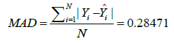
According to the formula above and Mean Absolute Deviation (MAD) test result the fitting effect is good. Finally the residual-fit predicted values scatterplot is as follows (Figure 1).

Figure 1: Residual-fit predicted values scatterplot.
According to the above test results this model can exclude the influence of multicollinearity and pass the endogeneity and heteroscedasticity tests therefore our model can be greatly explained by those explained variables.
According to the research the explanatory variable AAR is the influencing factor of real estate price which validates the H0 hypothesis in section model setting and there is a significant correlation between real estate price and AAR. Besides our proposed model can pass the endogeneity and heteroscedasticity tests so that we can hold this model. At the same time the MAD test value of the model in this paper is 0.28 and the MAD value is low which proves that the model has a high goodness-of-fit. Briefly concluding the average area per room has strong effect on the housing price in China.
In conclusion, our paper’s primary contribution is that it expands the empirical research on real estate price in China which finds out and proves a key factor influencing housing price. We believe that our paper will provide ideas for relative studies in the future. However this paper still has some significant drawbacks. Firstly our model is based on the classical regression models which may be too simple and requires more advanced algorithm for a more comprehensive relationship model to be built. Secondly the dataset only covers data from 2014 to 2018 and merely includes information from 34 cities which is apparently not enough from the view of both time range and population diversity. To address this issues further research could expand in these following areas including collecting datasets from official governmental websites or economic research websites which are more authoritative so that they may cover the fuller and more accurate dataset from 1998 when the housing reform was put into effect until now and they will contain information from hundreds of cities in China. Then a more extended time period and higher population diversity are covered to improve the integrity of the dataset. Last but not least we can use more advanced machine learning models to conduct relationship modelling between housing price and its influencing factors of higher complexity, which will describe the relationship between real estate price and its relative factors more precisely.
The authors declare that they have no conflict of interest.
The authors did not receive support from any organization for the submitted work.
Citation: Rong R, Liu Y, Li Z, Li S, Li J (2024) Empirical Analysis of Average Area per Room and House Price based on Two-way Fixed Effects Model-Evidence from China. J Stock Forex. 11:262.
Received: 04-Jun-2024, Manuscript No. JSFT-24-32051; Editor assigned: 06-Jun-2024, Pre QC No. JSFT-24-32051 (PQ); Reviewed: 20-Jun-2024, QC No. JSFT-24-32051; Revised: 27-Jun-2024, Manuscript No. JSFT-24-32051 (R); Published: 04-Jul-2024 , DOI: 10.35248/2168-9458.24.11.262
Copyright: © 2024 Rong R, et al. This is an open-access article distributed under the terms of the Creative Commons Attribution License, which permits unrestricted use, distribution and reproduction in any medium, provided the original author and source are credited.