Advances in Automobile Engineering
Open Access
ISSN: 2167-7670
ISSN: 2167-7670
Research Article - (2016) Volume 5, Issue 1
Fuel efficiency in hybrid electric vehicles requires a fine balance between combustion engine usage and battery energy, using a carefully designed control algorithm. Owing to the transient nature of HEV dynamics, driving conditions prediction, have unavoidably become a vital part of HEV energy management. The use of vehicle onboard telematics for driving conditions prediction have been widely researched and documented in literature, with most of these studies identifying high equipment cost and lack of route information (for routes unfamiliar to the GPS) as factors currently impeding the commercialization of predictive HEV control using telematics. In view of this challenge, this study inspires a look-ahead HEV energy management approach, which uses time series predictors (neural networks or Markov chains), to forecast future battery state of charge, for a given horizon, along the optimal front (optimal battery state of charge trajectory). The primary contribution of this paper is a detailed theoretical appraisal and comparison of the neural network and Markov chain time series predictors over different driving scenarios (FTP72, SC03, ARTEMIS U130 and WLTC 3 driving cycles). Based on the analysis performed in this study, the following useful inferences are drawn: 1. Prediction accuracy decreases massively and disproportionately on average with increased prediction horizon for multi-input neural networks, 2. In a single-input/single-horizon prediction network, the performance of both the neural network and Markov chain predictors are similar and near optimal, with a mean absolute percentage error of less than 0.7% and a root mean square error of less than 0.6 for all driving cycles analysed, 3. Markov chains appeal as a promising time series predictor for online vehicular applications, as it impacts the relative advantage of high precision and moderate computation time.
<Keywords: Time series prediction; HEV predictive control; Markov chains; Neural networks; Stochastic prediction; Hybrid electric vehicles; Intelligent control; Look ahead control
General Nomenclature
NEDC New European driving cycle
FTP Federal Test Procedure
WLTC Worldwide harmonized Light duty driving Test Cycle
US United States
NYCC New York City Cycle
IM Inspection and Maintenance
SC Supplementary driving Cycle
LA Los Angeles
ARTEMIS Assessment and Reliability of Transport Emission Models and Inventory Systems
HWFET Highway Fuel Economy Test
HEV Hybrid Electric Vehicle
SOC State of charge
MAPE Mean Absolute Percentage Error
RMSE Root Mean Square Error
GIS Geographic Information System
GPS Global Positioning System
In comparison to conventional vehicles, hybrid electric vehicles (HEVs) offer a number of advantages. The most popular of such advantages is the possibility of downsizing the original internal combustion engine, whilst meeting the power demand at the wheels. This advantage stems from the HEV being able to simultaneously deliver power to the wheels from both the internal combustion engine and the electric motor, thus resulting in reduced fuel consumption. The introduction of an electric driveline in an HEV also allows for kinetic braking energy regeneration. Aside from fuel consumption related advantages, the use of HEVs also presents the possibility of cranking the engine with the electric motor, which allows for the removal of the starter motor from the powertrain. This new cranking procedure will allow for a faster, smoother and a more improved cranking technique, as in the case of inertia cranking [1].
Crucial to achieving the aforementioned advantages, is a real time control strategy capable of coordinating the on-board power sources in order to maximize fuel economy and reduce emissions. Owing to the transient nature of HEV dynamics, driving conditions prediction have unavoidably become a vital part of HEV control. At present, two main methods exist to identify and predict future driving conditions. The first method is the use of traffic environment information provided by the GPS, or GIS [2-4], while the second method is the use of driving information gathered by on-board sensors. In the first approach, traffic environment information such as congested routes and arrival time can be provided for the driver to choose the best route. In addition, the use of look-ahead information, allows the HEV to plan how and when to use the stored energy in the battery and how to recharge it. Using this approach, Chan [5] reported a fuel savings of 15% for a prediction horizon of 500 meters.
Despite the advantages associated with vehicle telematics, they suffer from limitations: including equipment costs and lack of route information for routes unfamiliar to the GPS. The second method in comparison, offers a more realistic and viable approach to driving information identification as it relies only on the theoretical study of past driving patterns. Lin et al. [6] and Won et al. [7] were both able to incorporate driving pattern identification in the form of analysis of feature parameters (extracted from velocity data) to the receding horizon control of a hybrid electric vehicle. The reported control results are impressive, thus forming a paradigm for further application of driving pattern recognition to HEV control.
The use of time series predictive techniques for driving pattern recognition and prediction in vehicular applications has become increasingly popular of recent, with neural networks topping the list [8-14]. Through appropriate training and adjustment of weights, an artificial neural network can approximate any continuous measurable function to a desired accuracy. The use of Markov chain models as a method for vehicular time series prediction is relatively new and has only been reported by a few literature [9,10,12], with most of them focusing only on its preliminary theoretical frame work. Unlike any existing study, this paper offers two major original contributions to the related literature. First, a detailed theoretical framework for neural networks and Markov chains is developed. Next, the prediction accuracy of both methods over different driving scenarios (FTP72, SC03, ARTEMIS U130 and WLTC 3 driving cycles) are quantified and compared, with inferences drawn to explain the impact of prediction horizon on the accuracy of the compared predictors and the impact of network input on the prediction accuracy of neural networks. This comparative analysis is also extended on a subjective basis to recommend a promising time series forecasting approach for vehicular energy management applications.
Although the foregoing novel contributions are made specifically for the receding horizon energy management of hybrid electric vehicles, the theoretical bases of the observations made and inferences drawn still hold true for other time series prediction applications.
The disposition of this paper is as follows: first, the predictive control problem in HEV is introduced alongside the applicable assumptions. Next, the theoretical frame work for Markov chains and neural networks are developed in details, highlighting the key assumptions that apply to each method. Afterwards, both approaches are used over different horizons to predict the optimal battery state of charge trajectory of a parallel hybrid electric vehicle over different driving scenarios. Finally, the prediction accuracy of both methods is compared and useful explanations given to observed trends.
HEV predictive control problem
One imperative question during HEV control, is that of when and how to use the auxiliary energy which comes from the battery. In previous time series prediction inspired literatures [9-12], the proposed approach was to predict future vehicle velocities using neural networks or Markov chains. The predicted velocities are then compared to a database containing many driving segments, modeled from previous vehicle trips. The most similar segment to the one predicted is selected and its optimal control results (pre-calculated offline using dynamic programming) are applied. Although this approach has been reported to yield promising fuel savings [10], it’s control performance is limiting in the sense that it depends both on the size of the offline driving database, and the cycle identification algorithm in use.
In light of the prevalent challenge, this paper inspires a lookahead energy split approach which uses time series predictors (neural networks or Markov chains) to forecast future battery state of charge for a given horizon, along the optimal front (optimal battery state of charge trajectory).
Over different driving cycles as shown in Figures 1-4, the optimal dynamic programming model of a parallel HEV (see Appendix 1 for vehicle specification and Figure 5 for vehicle layout), developed in a previous study [15] is simulated to obtain the optimal battery state of charge trajectory. The obtained trajectories are then combined and used to train and validate the time series predictors (neural networks and Markov chains). The training and validation dataset is made up of a total of 10 standard driving cycles including, NEDC, JAPAN 1015, US06, LA92, NYCC, IM240, ARTEMIS U150, WLTC 1, WLTC 2 and HWFET.
The driving characteristics represented by the 14 driving cycles used in this study are comprehensive in an average sense, as it accounts for moderate urban driving scenarios (IM240 and WLTC 3 driving cycles), aggressive urban driving scenarios (LA92 driving cycle), calm highway driving scenarios (HWFET driving cycle) and aggressive highway driving scenarios (US06 driving cycle).
Prediction philosophy
The prediction network in this study as shown in Figure 6, has0 been set up to accommodate multi-input/multi-horizon prediction problems. At the beginning of each prediction problem, depending on the selected prediction network, the battery state of charge values used to initialize the network is measured online from the hybrid electric vehicle. These values are symbolically represented for different networks thus: A (Figures 6a and 6b); A and B (Figure 6c and 6d); A, B and C (Figures 6e and 6f). Using these initialized values, the first future battery state of charge is predicted along the optimal front for the different networks thus: B (Figures 6a and 6b); C (Figures 6c and 6d); D (Figures 6e and 6f). For multi-horizon prediction problems, the prediction for subsequent horizons (C and F (Figure 6b); D (Figure 6d); E (Figure 6f) are made using past immediate values from the prediction network. At the end of each prediction cycle (over the selected prediction horizon), the next battery state of charge value is assumed known and measured online from the hybrid electric vehicle (C and E (Figure 6a); D (Figure 6b); D and F (Figure 6c); E (Figure 6d and Figure 6e); F (Figure 6f). This measure has been implemented for error reduction reasons.
Neural networks theoretical frame work
Neural networks can be trained to learn a highly nonlinear input/ output relationship by adjusting weights to minimize the error between the actual and predicted output patterns of a training set [16]. This form of supervised learning is facilitated by the back propagation method (shown in Figure 7), which could be articulated in the following steps:
Feed forward approach
i. Using inputs (X1 and X2) to the prediction network, calculate the input to hidden layer neurons.

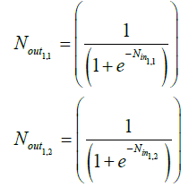
ii. Calculate the output from hidden layer neurons

iii. Calculate the input to the output neuron

iv. Calculate the output from the neural network

v. Calculate the prediction error
Yactual - Yp = error
Back propagation approach
Calculate local gradients of output and hidden layers
 (8)
(8)
 (9)
(9)
i. Adjust the weight of the network using the gradient descent learning rule
 (10)
(10)
 (11)
(11)
 (12)
(12)
 (13)
(13)
 (14)
(14)
 (15)
(15)
ii. Using the recomputed weights perform steps 1 – 7 again while 
Note: Steps 1 to 8 could be applied to networks with more inputs, hidden layers and outputs.
Summarily, the back propagation algorithm adjusts the weights of each unit in such a way that the error between the desired output and actual output is reduced. This process requires the computation of error derivative for each weight, which is a measure of how the error changes as each weight is increased or decreased.
In this study, 80% of the optimal battery state of charge data is used for neural network training, while 20% is used for performance validation. The neural network set up in this study, allows for multi inputs and a single output. Understanding the impact of hidden layers on the performance of neural networks is outside the scope of this study and as such 20 hidden layers are applied to the whole prediction network. It is assumed that the comparative analysis contributed by this study is unaffected by the number of hidden layers used, provided the same number of layers are maintained throughout. The network notations are defined in Table 1.
| Wx 1,1 Wx 1,2 Wx 2,1 Wx 2,1 |
Randomly generated input weights |
X1 X2 |
Inputs to neural network |
| N1,1 N1,2 |
Neurons in hidden layer nodes |
Nin 1,1 Nin 1,2 |
Inputs to hidden layer neurons. |
| α | Learning rate | Nout 1,1 Nout 1,2 |
Outputs from hidden layer neurons |
| δN 1,1 δN 1,2 δy |
Local gradients | WN 1,1 WN 1,2 |
Randomly generated hidden layer weights |
| Yin | Input to output neuron |
YP | Predicted output |
Table 1: Notation definition for an artificial neural network predictor.
Markov chains theoretical frame work
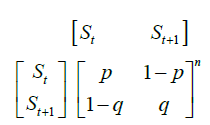
A Markov chain is a collection of random variables having the property that given the present, the future is conditionally independent of the past. A one step state transition in a Markov chain model could be described using a state transition diagram, shown in its simplest form in Figure 8. Mathematically, this one step state transition diagram could be adapted to account for transition probabilities between different states, for each prediction horizon thus:
 (16)
(16)
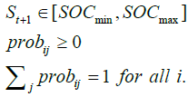
The resulting matrix is known as the transition probability matrix. The transition probability matrix maps the probability of occupying a new state based on the current state. Mathematically, the transition probability matrix consists of K by K matrix whose entries record the probability of moving from one state to another. In this study, the transition probability matrix is estimated on the basis of simulation results from 10 standard driving cycles which represent mixed city and high way driving at different aggressively levels. The combined optimal battery state of charge trajectory for all 10 driving cycles is mapped in to the sequence of quantized states using the nearest-neighbours method with a resolution of 0.01. The transition probabilities making up the transition probability matrix is estimated using the maximum likelihood estimation method expressed mathematically in Equation 17.
 (17)
(17)
The resulting transition probability matrix (TPM) for this study is shown graphically in Figure 9.
For each prediction horizon, state transition is based on the future state with the highest transition probability (calculated mathematically using Equation 18, and detailed graphically in Figure 10 for this study).
 (18)
(18)
Where:

The Markov chains model used in this study homogenous and time invariant.
In this section, the predictability of both neural networks and Markov chains are investigated over the FTP72, SC03, ARTEMIS U130 and WLTC 3 driving cycles. These cycles are different from the ones used for the initial training, and as such offer an unbiased appraisal of both methods.
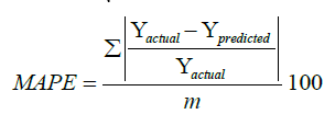
For both predictors, the prediction philosophy introduced in section 2.2 is applied. The least root mean square error (RMSE) (Equation 19) and mean absolute percentage error (MAPE) (Equation 20) metrics are used to assess the prediction accuracy of both predictors. RMSE as the name implies, provides a quadratic loss function as it squares and subsequently averages the prediction errors. Such squaring gives considerably more weight to large errors than smaller ones. MAPE on the other hand, is a relative measure which expresses prediction errors as a percentage of the actual data. This metric provides an easy and intuitive way of comparing errors between two predictors.
 (19)
(19)
 (20)
(20)
Where: “Yactual” is the actual value, “Ypredicted” is the predicted value, “m” is the number of data points.
Neural networks
In Figures 11 and 12, the impact of neural network inputs on MAPE and RMSE respectively, is investigated.
From these plots, MAPE and RMSE are found to increase massively and disproportionately on average as the prediction horizon increases for multi-input neural networks.
To explain this trend, the impact of neural network input on error build up is investigated over part of the US06 driving cycle, as shown in Figure 13. In this example, the network with 2 inputs and 1 prediction horizon (Figure 13a) has the lowest prediction error at node E, owing to low error contribution from node C. Similarly, the network with 2 inputs and 2 prediction horizons (Figure 13b) has 2 error contributing nodes (B and C) which further increase the prediction error at node E. The same explanation also holds for the network with 2 inputs and 3 prediction horizons (Figure 13c) which has 3 error contributing nodes (A, C and D).
In summary, for multi-input neural networks, the error observed at each prediction stage is a cumulative effect of the error in the inputs leading to that stage. A buildup of this contributive error throughout the prediction stages, results in the overall prediction error observed.
Comparison between Markov chains and neural networks
Prediction accuracy: In this section, the prediction precision of Markov chains and neural networks are compared over the FTP72, SC03, ARTEMIS U130 and WLTC 3 driving cycles, using the MAPE and RMSE criteria as shown in Figures 14 and 15. To maintain comparative fairness, both predictors have been set up on the basis of single-input/ single-output. The resulting plots show that both predictors have a similar level of performance, and command a high level of prediction precision, even at long prediction horizons, with a root mean square error of less than 0.6 and a mean absolute percentage error of less than 0.7% for all driving cycles analysed.
The low RMSE and MAPE values observed for each predictor, over different driving scenarios imply that both predictors offer an accurate estimation of the future battery state of charge, even at long prediction horizons. A visualizeable time series confirmation of this observation over the ARTEMIS U130 driving cycle is detailed in Figure 16.
Computation time and complexity: Neural networks learn by iterative weight adjustments through hundreds of hidden layer nodes in each prediction horizon and as such learn slower than Markov chains. By using random weights for pattern learning (Section 2.3, Equation 7), the prediction performance of neural networks are non-repeatable, though similar.
With little or no difference in the prediction precision of both predictors, Markov chains appeal as a promising time series predictor for online vehicular applications, as it impacts the relative advantage of high precision and moderate computation time.
This paper inspires a look ahead HEV energy management approach which uses time series predictors (Neural networks or Markov chains) to forecast future battery state of charge for a given horizon, along the optimal front (optimal battery state of charge trajectory).
The primary contribution here is a detailed theoretical appraisal of the neural network and Markov chain time series predictors over different driving scenarios (FTP72, SC03, ARTEMIS U130 and WLTC 3 driving cycles), with a view to understanding:-
1. The prediction accuracy of both predictors in vehicular energy management applications.
2. The impact of prediction horizon on the accuracy of both predictors.
3. The impact of network inputs on the prediction accuracy of neural networks.
From the obtained results, the following useful inferences are drawn:
1. Prediction accuracy decreases massively and disproportionately on average with increased prediction horizon for multi-input neural networks. Error build up in the network inputs through different horizons, is responsible for this trend.
2. In a single-input/single-output prediction network, the performance of both predictors are similar and near optimal with a mean absolute percentage error of less than 0.7% and a root mean square error of less than 0.6 for all driving cycles analysed.
This study formulates a successful template for the application of a time series predictor (neural networks or Markov chains) to a look ahead HEV control strategy. Building on the theoretical framework developed in this study and leveraging on the relative advantage of the Markov chains predictor (high precision and moderate computation time), future work will see to the realization of a Markov chains inspired online receding horizon HEV control strategy.