Poultry, Fisheries & Wildlife Sciences
Open Access

Impacts of Climate Variability on the Pink Shrimp (Penaeus subtilis) Fishery on the Amazon Shelf

Author info »

Introduction

Marine shrimp fisheries are an important component of the world fisheries landing, and in Brazil. Shrimp fisheries in tropical and subtropical regions are highly productive [1]. The life cycle and the spatial and temporal distribution patterns of the penaeids are influenced by several environmental factors, such as: temperature, salinity, substrate type, water depth, tides, and food availability, which together determine recruitment patterns and the health of stocks [2-7]. The Southern brown shrimp, Farfantepenaeus subtilis (Pérez Farfante), together with Farfantepenaeus brasiliensis, contribute 95% of the total landing of marine shrimp fisheries on the continental shelf of northern Brazil [8]. This fishery uses a bottom trawling system the double rig system, which consists of two trawls with two otter boards, coupled to two warps controlled by motorized winches [8,9]. The industrial trawling fleet that targets Southern brown shrimp in northern Brazil uses boats of 20 m-28 m in length, with autonomy of approximately 37 days. All these vessels are equipped with a Global Position System (GPS), echo sounder, radar and sonar, and freezer compartments [9,10]. Despite the economic importance of industrial shrimp fisheries on the northern coast of Brazil, few studies have evaluated the variability in the productivity of this resource, and there are few data on the relationship between Southern brown shrimp fishery productivity and marine climate variability for nay region. This hampers the development of effective fishery management strategies. The present study provides the first systematic analysis of the influence of climate on shrimp fishery productivity in the region of the continental shelf of northern Brazil, relating the variability in productivity to the cycle of the marine climate.

Materials and Methods

Study area

The study area is located on the Amazon shelf (latitudes 0˚40’S and 4˚33'N and longitudes 51˚15’W and 47˚25’was shown in Figure 1. The climate is tropical humid influenced by the hydrological cycle of the Amazon River, which includes a flooding season, from December to May, and a dry season, from July to November. These periods typically coincide with the intensity of local rainfalls. The mean Sea Surface Temperature (SST) varies from 27˚C in the dry season, to 24˚C in the rainy season. The Southeast Trade Wind is the dominant wind and is more intense at the dry season onset [11].

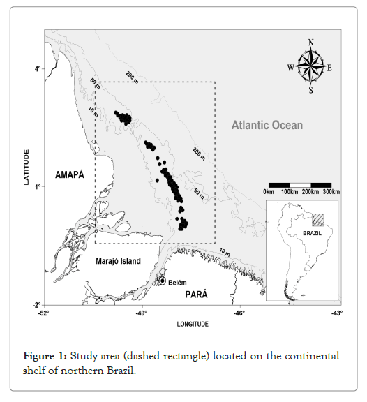
Figure 1: Figure 1: Study area (dashed rectangle) located on the continental shelf of northern Brazil.

Data

Monthly oceanographical and meteorological data for the continental shelf of northern Brazil are from the National Center for Environmental Prediction/National Center for Atmospheric Research, and the Reanalysis Project, N/N Reanalysis and Reanalysis 2 [12,13]. The monthly means were distributed in a Gaussian grid with a spatial resolution of 1.8758˚ × 1.9058˚ and included data anomalies of the zonal (u) and meridional (v) surface wind, rainfall (RAIN), and Sea Surface Temperatures (SST). Monthly data on the flow of the Amazon River (ARD, m3•s^-1) were also read from Brazilian National Water Agency. Two temporal series of climatological indices, the Oceanic Nino Index (ONI) and the Gradient Inter-hemispheric SST in the Atlantic Index (GITA) were also included here. We read the ONI time series. We calculated the GITA index by the difference between the SST anomalies in the North and South Atlantic Ocean [14]. We estimated the normalized anomalies of all the environmental parameters for the study period (January 2010 to December 2016) to make the nondimensional data mutually comparable. The climatology data are available in the Climate Data Assimilation System.

Catch Per Unit of Effort (CPUE)

The monthly shrimp landings were estimated from the total landings (in t) from AMASA (Amazonia Industria de Alimentos Sociedade Anonima) the largest shrimp fishery company in Belem. It accounts for nearly 80% of the total shrimp processing in the state of Para. The fishing CPUE was calculated by the catch per fishing days (ton) at sea. Shorter trips take place at the beginning of the fishing season and the longer ones at the end of the production year discounting the fishing ban [9,10]. AMASA landing time series ranges from January 2010 to December 2016.

The fisheries

The industrial shrimp fishing is carried out by the double-drag system, with otter twin trawls and two control otter boards in each net coupled to two lateral mechanical arms, called "tangones", controlled by motorized winches with cables and net tractions fixed at the end [9,10]. The main dimensions gears in this region are: 17 m in length and 22 mm between knots in the bagger net. The “mixer”, a steel chain connected to the front end of the door base, 20 m defines the net opening. The doors were rectangular in shape, made of wood and iron, 2.5 m long and 1.15 m wide and approximately 150 kg in weight.

The fishing ban

From 2010-2016, the Southern brown shrimp fishing ban period in the Brazilian north coast, was regulated through the Normative Instructions of the Ministry of the Environment of Brazil (MMA) and in the then Ministry of Fisheries and Aquaculture (MPA). In the 2010 fishing season, the ban period was from October 15 to February 15, determined by MMA Normative Instruction N˚09, from September 14, 2004. In the following year, the Interministerial Normative Instruction No. 14, from October 31, 2011, determined the fishing ban between December 15 and February 15. In 2012 and 2013 the ban period continued albeit governed by the MPA-MMA Interministerial Normative Instruction No. 15, of November 28, 2012. From 2014 to 2016, the ban was defined again by MMA Normative Instruction No. 09, of September 14, 2014, which determined it from October 15 to February 15. After 2010, an exceptional fishing concession for the Southern brown shrimp fleet, allowed it not being idle during the ban (Normative Instruction No. 2 of January 15, 2010).

AMASA has a Federal Inspection Seal (SIF) allowing it to market its products with several countries. It has its own shrimp fleet and buys the production from others. During the legal shrimp fishing season this company also processes fish in its production line, mainly King weakfish (Macrodon ancylodon).

Statistical analyses

When some of our variables are highly correlated we can choose to disregard one or some of them in order not to repeat our interpretations. We use here a robust statistical method [15], Pearson's correlation and scatterplot, to test the collinearity between all the variables studied here, in order to avoid possible distortions in our results inferences as well as weak conclusions. When some of our variables are highly correlated we can choose to neglect one or some of them. The results of Pearson's correlation analysis are seen in Table 1 and Figure 2. The analysis indicates that rainfall (RAIN) is correlated with ENSO events or ONI index (cc=0.52). After collinearity tests, the environmental variables used here were reduced to: Amazon River Flow Anomaly (ARD); Zonal (u) and meridional (v) wind components; Sea Surface Temperature (SST); ONI and GITA climate indices.

Table 1: Pearson correlation coefficients.

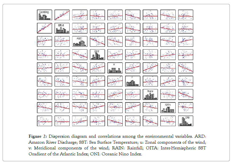
Figure 2: Dispersion diagram and correlations among the environmental variables. ARD: Amazon River Discharge; SST: Sea Surface Temperature; u: Zonal components of the wind; v: Meridional components of the wind; RAIN: Rainfall; GITA: Inter-Hemispheric SST Gradient of the Atlantic Index; ONI: Oceanic Nino Index.

We calculated a multiple regression analyses where the response variate (Y) is the monthly fishing landings and effort. The independent continuous variates are:

1. Zonal wind (u, m/s);

2. Meridional wind (v, m/s);

3. Sea surface temperature (SST, ˚C);

4. Ocean El Nino Index (ONI);

5. Gradient Interhemispheric Sea Surface Temperature in the Atlantic Ocean index (GITA) and

6. River discharge (ARD, m³/s). Residual analyses were performed in order to validate the model. The calculations were performed using the R program (R Core Team) [16].

Multiple Linear Regression (MLR) is a technic which assumes that the response variable (landings or effort, separately) is directly related to a linear combination of the explanatory variables (meteorological and oceanographic). We adopted a twofold choice: (i) with and without a stepwise procedure when considering the shrimp landings as dependent variate; (ii) performing just a stepwise procedure when the fishing effort as dependent variate.

Cross wavelet analysis compares wavelet spectra of the two series. This allows similarities detection between two local fluctuations in time series and the phase estimation between these fluctuations. In order to detect significant results, we located the red noise inside the cone of influence with the same coefficients of the first order auto regression [17]. The cone of influence on the scalograms indicates the region not influenced by the edge effects. While analyzing wavelet cross-power spectrum emphasizes the commonness of the two series, the wavelet coherence emphasizes the correlations between these series, i.e. the coherence fluctuations. The technical details may be found in Grinsted et al. and Torrence and Compo [17,18]. This analysis seeks to find out the local correlation of the significant oscillations observed between the fishery and environmental variables.

The Redundancy Analysis (RDA) is a multivariate statistical method used to estimate the linear relationships between blocks of variables [19,20]. In the present study, the explained matrices are the monthly shrimp landing. The explanatory matrices are the seven variates above. The statistical significance (p ≤ 0.05) of these tests was calculated by a Monte Carlo analysis with 9999 permutations using the Canoco for Windows 4.54^® [20].

Results

Southern brown shrimp fishery production variability

During the studied period largest landings were recorded in May 2011, 2013, 2014, and 2015, albeit the landings from July 2013 and June 2015 were also relatively high. Landings (Y) increased with the effort (f), with exception in 2016. In 2014 and 2016, however, there was a 1-2 months lag between these variables as shown in Table 2, although the peak in those two years still occurred during the rainy season. There was a 2 to 3 months lag between the peak of the shrimp landings in relation to the negative peak of the GITA. The peak was also related to the southward heat flow in the Atlantic Ocean, i.e. the negative phase of the GITA as shown in Table 3.

Table 2: Months in which the Southern brown shrimp landings and Amazon River discharge between 2010-2016.

Table 3: Southern brown shrimp production and GITA, that is, northward (positive) and southward (negative) flow between 2010-2016.

Analyzes linking the shrimp fishery production and climate variability

Table 4 shows the MRL without stepwise procedure results, considering the landings as the dependent variate and YEAR as a factor. Tables 5 and 6 show the MRL stepwise results, considering the landings (Y) and the fishing effort (f) as dependent variates and independent variates respectively.

(Intercept) 

Year 2011 

0.180 

Year 2012 

0.479 

Year 2014 

Year 2015 

Year 2016

16.929

f               

v 

Table 4: Linear multiple regression results for the monthly shrimp fisheries landings (Y).

Table 5: Stepwise multiple regression results for the monthly shrimp fisheries landings (Y).

(Intercept) 

v              

GITA 

Table 6: Stepwise multiple regression results for the monthly shrimp fisheries landings (Y).

Landing model without stepwise procedure

Heuristically we chose a three variables model (meridional wind component (v), YEAR and fishing effort (f)) expressed by Equation 1:

LANDING=-14.733+0.233×f –10.913×v+YEAR

The Table 4 shows the year 2016 and fishing effort with significant statistical results (p<0.01) on linear multiple regression for the monthly shrimp fisheries landings. The Figure 3 (a, b and c) shows that fishing landings are positively related to fishing effort (f) and negatively related to the meridional wind component (v), normal distribution of residues, based on the Shapiro-Wilk test (w=0.988, p-value=0.855, n=56).

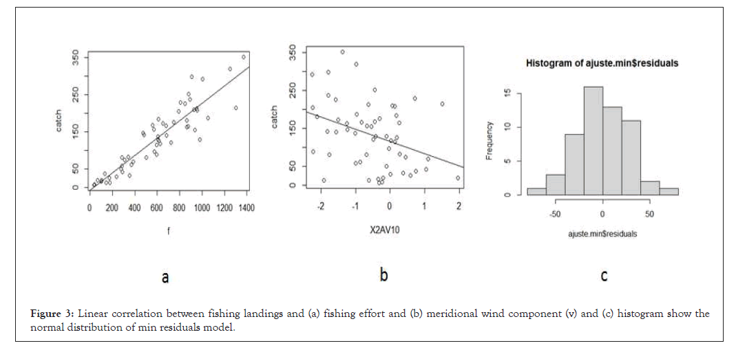
Figure 3: Linear correlation between fishing landings and (a) fishing effort and (b) meridional wind component (v) and (c) histogram show the normal distribution of min residuals model.

Landing model with stepwise procedure

The final model expressed by Equation 2, three explanatory variables (sea surface temperature (SST), meridional wind component (v) and fishing effort (f)):

LANDING=2.7461-9.0269×SST-8.8483× v + 0.2299×f

Where R2=0.8612, N=56.

The Table 5 shows that only effort had significant result (p<0.01) when tested by stepwise multiple regression for the monthly shrimp fisheries landings. The Figure 4 shows observed data of Southern brown shrimp fisheries landings and adjusted data from the proposed MRL model. It should be noted that, although some adjustments are not satisfactory, especially the peak landing values, the trend of the observed and adjusted values is similar.

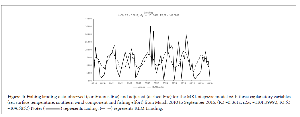
Figure 4: Fishing landing data observed (continuous line) and adjusted (dashed line) for the MRL stepwise model with three explanatory variables (sea surface temperature, southern wind component and fishing effort) from March 2010 to September 2016. (R2 =0.8612, s2xy =1101.39990, F2,53 =104.5852) Note: () represents Lading, () represents RLM Landing.

Effort model with stepwise procedure

The final model chose two explanatory variables, the southern component of the wind () and the heat flow in the Atlantic Ocean (GITA), expressed in Equation 3:

EFFORT = 613.32 - 50.74×v – 56.03×GITA + ε

The Table 6 shows that GITA was the only variable that had significant statistical result (p<0.01) of effort variability. Fishing effort is negatively related to the meridional wind component (v) (Figure 5a). The Figure 5b showed normal distribution of residues, based on the Shapiro-Wilk test (w=0.978, p-value=0.386, n=56). The Figure 6 shows the observed and adjusted fishing effort. The model fits satisfactorily over the period considered from 2010 to 2016.

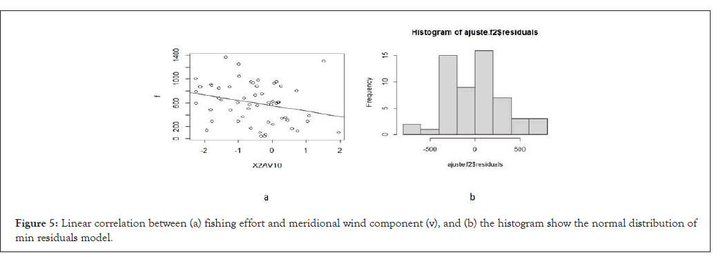
Figure 5: Linear correlation between (a) fishing effort and meridional wind component (v), and (b) the histogram show the normal distribution of min residuals model.

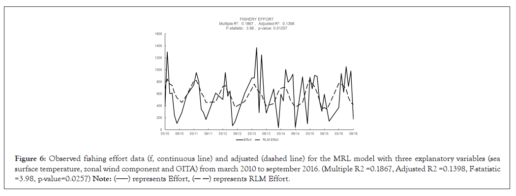
Figure 6: Observed fishing effort data (f, continuous line) and adjusted (dashed line) for the MRL model with three explanatory variables (sea surface temperature, zonal wind component and GITA) from march 2010 to september 2016. (Multiple R2 =0.1867, Adjusted R2 =0.1398, F-statistic =3.98, p-value=0.0257) Note: () represents Effort, () represents RLM Effort.

Cross-wavelet analysis

The cross-wavelet analysis of the mutual variability between the Southern brown shrimp landing and the SST indicated one peak of energy in 8 months advanced with the phase at 135˚, i.e. the Southern brown shrimp landing responds in approximately 3 months (3/8 of the peak energy period) to the shifts in the SST (Figure 7). Analyzing the cross-wavelet between the effort and the SST showed the peaks of energy similar of the effort and u analysis, i.e. an annual peak and another centered in 1.5 years. The annual peak is in phase, while the second peak is lagged with the phase at 270˚e, i.e. the effort responds in approximately 4 months to the SST variability (Figure 8). While the cross-wavelet analysis between the effort and GITA events indicate an annual peak in energy in the opposite phase (Figure 9). The coherence spectrum has the same phases as those observed in the cross-wavelet.

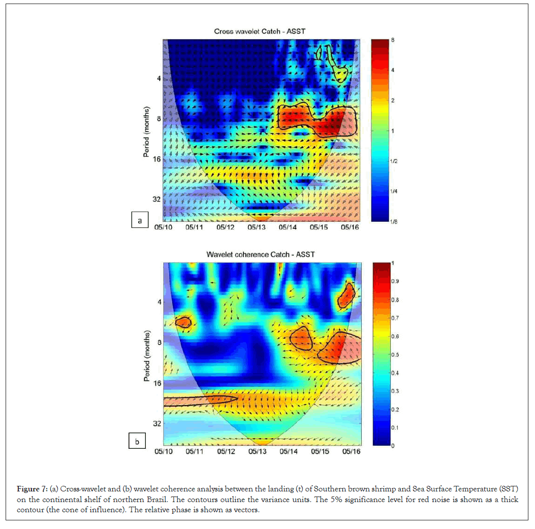
Figure 7: (a) Cross-wavelet and (b) wavelet coherence analysis between the landing (t) of Southern brown shrimp and Sea Surface Temperature (SST) on the continental shelf of northern Brazil. The contours outline the variance units. The 5% significance level for red noise is shown as a thick contour (the cone of influence). The relative phase is shown as vectors.

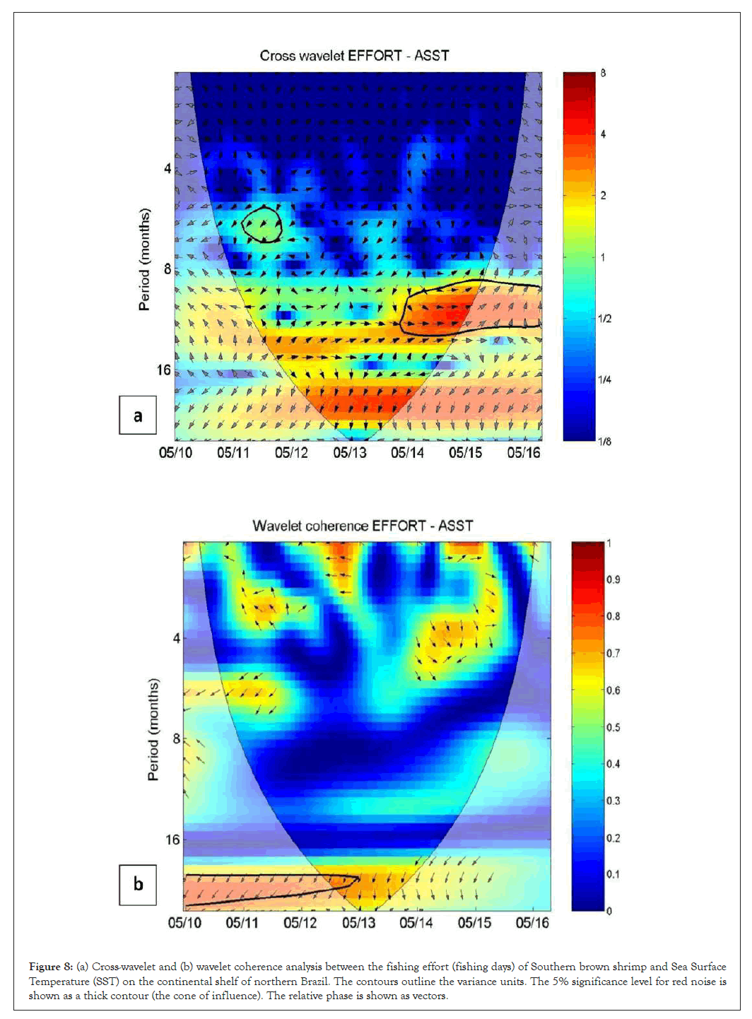
Figure 8: (a) Cross-wavelet and (b) wavelet coherence analysis between the fishing effort (fishing days) of Southern brown shrimp and Sea Surface Temperature (SST) on the continental shelf of northern Brazil. The contours outline the variance units. The 5% significance level for red noise is shown as a thick contour (the cone of influence). The relative phase is shown as vectors.

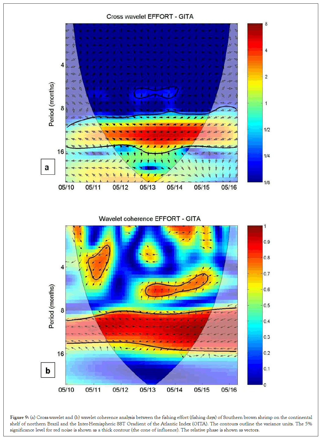
Figure 9: (a) Cross-wavelet and (b) wavelet coherence analysis between the fishing effort (fishing days) of Southern brown shrimp on the continental shelf of northern Brazil and the Inter-Hemispheric SST Gradient of the Atlantic Index (GITA). The contours outline the variance units. The 5% significance level for red noise is shown as a thick contour (the cone of influence). The relative phase is shown as vectors.

The relationship between the southern brown shrimp landings and climatic variability

The Redundancy Analysis (RDA) was used to model the relationships between Southern brown shrimp production, as described by the CPUEs and shrimp landings, and the climatic variability on the continental shelf of northern Brazil, as defined by the environmental variables. In the plot (Figure 10), the angle between the black and red arrows represents the degree of correlation, with angles close to 0˚ representing a correlation close to 1, and angles closer to 180˚, a correlation close to -1. The length of the arrows is also proportional to the intensity of the correlation. The RDA shows that the CPUE was correlated positively with the Amazon River discharge (ARD) and Sea Surface Temperatures (SST). The shrimp landing was also correlated positively with the zonal wind component (u), while the CPUE and landings were correlated negatively with the Inter-Hemispheric SST Gradient of the Atlantic (GITA). The RDA model explained 69.7% of the variance in the landing and effort, considering four exploratory factors explained in the third canonical axis. Overall, then, four variables contributed significantly to the explanation of the model: ARD, SST, u, and GITA.

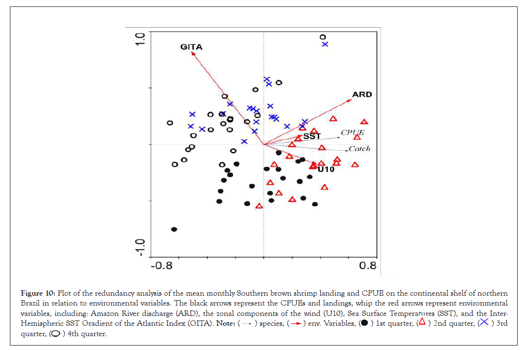
Figure 10: Plot of the redundancy analysis of the mean monthly Southern brown shrimp landing and CPUE on the continental shelf of northern Brazil in relation to environmental variables. The black arrows represent the CPUEs and landings, whip the red arrows represent environmental variables, including: Amazon River discharge (ARD), the zonal components of the wind (U10), Sea Surface Temperatures (SST), and the Inter- Hemispheric SST Gradient of the Atlantic Index (GITA). Note: () species, () env. Variables, () 1st quarter, () 2nd quarter, () 3rd quarter, () 4th quarter.

Discussion

Anthropogenic global warming has had profound impacts on physical and biological processes on both global and regional scales. Although the fishery production of Brazil represents only 0.5% of the world total, fisheries are an extremely important activity on both national and regional scales [21]. Fishery production may be affected by many factors in addition to fishing effort, such as climate and ocean variability, such as sea surface temperature, salinity, wind, turbulence, oxygen, hydrodynamics, air-sea interactions and climate events in meso and large scale.

As usual in industrial shrimp fisheries, the average proportion of shrimp tail in relation to the bycatch is 1:5 in weight. Species such as King Weakfish (Macrodon ancylodon) and Rake stardrum (Stellifer rastrifer), are predominant in the bycatch [22,23]. Industrial fishing for Southern brown shrimp occurs mainly between 40 m to 60 m depth. In other regions of the Earth there are great fluctuations in the landing of Southern brown shrimp [2]. The life cycle of shrimp is complex and short-lived.

The shrimp variability in the Alabama, Mississippi, Louisiana and Texas continental shelves show that the annual number and weight of the brown shrimp per trawl is positively correlated with annual Sea Surface Temperature (SST) averaged over the continental shelves [24]. Shrimp are more numerous in the summer and the correlation of April and May SST anomaly is much higher for the number and weight per trawl in the summer than in the fall.

Southern brown shrimps are subject to strong fluctuations in recruitment, which is governed by highly variable environmental conditions and thus influences the abundance of adult stocks [25]. The life cycle of Southern brown shrimp on the Amazon shelf indicates that it is extremely related to the dynamics of the hydrological cycle of the Amazon River. The Amazon River discharge is characterized by two seasons, the dry season between October and November and the full season between May and June [26,27]. Between the months of December and January, the flow of the river increases (flood) with a peak between May and June (full). Then, between the months of June and July, the flow will decrease (ebb) with its lowest level between October and November (dry). This discharge is responsible for maintaining the extensive substrate of mud and sand in this region. The river plume can go 300 km from the coast in the full season and 50 km in the dry season [28].

ENSO events (El Nino/Southern Oscillation) are considered by several authors as one of the main reasons for environmental variability in the tropics. In the Amazon region, phenomena of El Nino and La Nina contribute to the regulation of the hydrological cycle of the Amazon River. El Nino periods are warmer and drier, while La Nina periods are rainier and colder [26,29].

Individuals and populations are influenced by the variability of the local climate, by factors such as temperature, salinity, winds, currents and rain. Ocean-atmosphere interaction creates dynamic systems with complex patterns that can influence ecological processes in several ways. Southern brown shrimp, being a benthic species, should also be influenced by shallow water oceanographic processes in the Amazon shelf, barotropic and baroclinic processes, circulation and thermohaline gradient and sea and geostrophic currents, for example.

In this region the marine currents vary from 1.5 to 85 km.h^-1, according to the tide, requiring great knowledge from the master of the fishing vessel and the vessel's capacity to have a continuous control of the current, drag direction, substrate type and undersea relief [9]. The success of the lateral migration of juvenile shrimp from the nursery area to the open sea and subsequent recruitment to fishing, depends on a set of environmental conditions, such as; decreased discharge from the Amazon River; mild winds; increase in salinity, decrease in turbulence in the water column of the internal continental shelf in northern Brazil. Favorable environmental conditions for some year can lead to periods of high recruitment, contributing to the increase in landings for some months.

When Patos Lagoon (South of Brazil) discharge is below average, currents forced by SW winds can enhance larval transport into the estuarine area, leading to an increase in Southern brown shrimp captures [30]. Also, shrimp catches variability is related to ENSO events. They show wind can also impact production through its effect on the displacement of larvae from the spawning area.

Another factor that regulates the performance of shrimp fishing is the amount of diesel oil used by the industrial fishing vessel. This will define the fishing time allowed to remain at sea. This data is very important to have a better explanation of the variability of the Southern brown shrimp fishing effort.

The harvesting of the principal fishery resources in the Amazon region is related to the heat flow in the Atlantic Ocean, as indicated by the GITA [26,31]. These relationships are extremely complex and, are influenced by several other factors. For example, it was reported opposite results in relation to El Nino for blue shrimp fishing in California Bay [32].

The fishery variability is not easy to understand. It has an intrinsic net between the knowledge about the dynamic of each variable and a robust fishery dataset. The use different models with high significance statistic, like RLM, can allow for the conciliation of divergent conclusions and provide the necessary insight to simulation of predictions.

The fishing fleet vessels are among those with the greatest fishing power in the country, length around 20 meters and a sole engine with 425 HP [33]. As known trawling requires high fuel consumption, due to travelling longer distances and to the vessel's refrigeration system. Therefore, the fuel determines fishing trip duration, and the amount of fuel that must be available for the trip depends directly upon the availability of the ship-owners financial resources, since the diesel, represents around 60% total coasts [34].

In Figure 11, we present a logical schematic diagram to illustrate and summarize the results of this research regarding the relationships between Southern brown shrimp production, the environmental variables studied here and climatic variability. This diagram shows the variables and their direct or inverse relations indicated by the up or down direction, respectively, of the arrows.

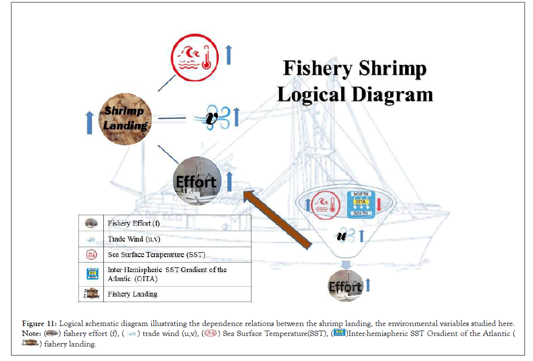
Figure 11: Logical schematic diagram illustrating the dependence relations between the shrimp landing, the environmental variables studied here. Note: () fishery effort (f), () trade wind (u,v), () Sea Surface Temperature(SST), ()Inter-hemispheric SST Gradient of the Atlantic () fishery landing.

Conclusion

Our results show that small and mesoscale events, such as sea surface temperature, the duration and intensity of the hydrological cycle and the field of winds, as well as large scale events, like ENSO and heat flux in the Atlantic Ocean, interact with the shrimp fishery dynamics in the study area. This is a new and especially relevant step to understand the spatial-temporal variability in landing of the Southern brown shrimp resource in the Amazon shelf.

However, the absence of more robust biological and fishing data shows that the mechanisms underlying this relationship are unclear. There is a growing need for the compilation of more extensive and reliable productivity and effort data, to ensure the development of more effective policies for the management go fishery resources. A long-term time series will be required to ensure the best interpretation of patterns, and the development predictive population models that integrate environmental parameters systematically.

Acknowledgements

The authors thank Mr Arnaldo and Ms Valeria from Amazonas Food Industry (AMASA) for releasing the fishing data used here. The environmental data was obtained from Brazilian National Water Agency (ANA) and NOAA/NCEP. Our thanks are also directed to Stephen Ferrari who helps us to produce the final English version of this paper. Author Contributions: BB, BM, ZN, WP delineated the study. WP, BM, BB collected the data. WP, BB, RC contributed with resources, analyzed the data and wrote the manuscript.

Sources of Funding

Sustainable By-catch Management of Shrimp Trawling in Latin America and the Caribbean-Project (REBYC II-LAC), funded by the United Nations Food and Agriculture Organization (FAO) and the World Environment Fund. Environment (GEF).

Conflict of Interest

All authors declare that the research was conducted in the absence of any commercial or financial relationships that could be construed as a potential conflict of interest.

References

1. Isaac VJ, Dias Neto J, Damasceno FG. Biology, population dynamics and fisheries management of the Southern brown shrimp Penaeus subtilis from northern Brazil. Série de Estudos de Pesca, Colecao Meio Ambiente, IBAMA, Brasília. 1992.
2. Dall W, Hill BJ, Rothlisberg PC, Sharples DJ. The biology of the Penaeidae. Adv Mar Biol 1990;27:1-489.

   [Crossref] [Google Scholar]

3. Fransozo A, Costa RC, Mantelatto FL, Pinheiro MA, Santos S. Composition and abundance of shrimp species (Penaeidea and Caridea) in Fortaleza Bay, Ubatuba, São Paulo, Brazil. In: Escobar-Briones E, Alvarez F. (Edn) Modern approaches to the study of Crustacea. Springer, Boston. 2002.
4. Costa RC, Fransozo A. Abundance and ecologic distribution of the shrimp Rimapenaeus constrictus (Crustacea: Penaeidae) on the northern coast of São Paulo State, Brazil. J Nat Hist 2004;38:901-912.

   [Crossref] [Google Scholar]

5. Castro RH, Costa RCD, Fransozo A, Mantelatto FL. Population structure of the seabob shrimp Xiphopenaeus kroyeri (Heller 1862) (Crustacea: Penaeoidea) in the littoral of São Paulo, Brazil. Sci Mar. 2005;69:105-112.

   [Crossref] [Google Scholar]

6. Aragón-Noriega EA. Coupling the reproductive period of blue shrimp Litopenaeus stylirostris Stimpson, 1874 (Decapoda: Penaeidae) and sea surface temperature in the Gulf of California. Ver Biol Mar y Oceanogr. 2007;42:167-175.

   [Crossref] [Google Scholar]

7. Castilho AL, Pie M, Fransozo A, Pinheiro AP, Costa RC. The relationship between environmental variation and species abundance in shrimp community (Crustacea: Decapoda: Penaeoidea) in south-eastern Brazil. J Mar Biol Ass. 2008;88:119-123.

   [Crossref] [Google Scholar]

8. Frédou FL, Mourão K, Barbosa C, Almeida O, Rivero S, Thompson R. Characterization of industrial fisheries on the North Coast of Brazil. Pap. NAEA 2009;237:1-33.
9. Aragón-Noriega JAN, Cintra IHA, Silva KC. Current situation of shrimp fishery on the amazon continental shelf. Acta Fish. and Aquat. Res. 2015;3:61-76. [Crossref]

   [Google Scholar]

10. Bentes B, Isaac VJ, Espírito-Santo RVD, Frédou T, Almeida MCD, Mourao K, et al. Multidisciplinary approach to identification of fishery production systems on the northern coast of Brazil. Biota Neotrop. 2012;12:81-92.

    [Crossref] [Google Scholar]

11. Fisch G, Marengo JA, Nobre CA. A general review of the climate in the Amazon. Acta amazona. 1998;28:101-101.

    [Crossref] [Google Scholar]

12. Ebisuzaki W, Kanamitsu M, Potter J, Fiorino M. An overview of Reanalysis-2. In: Proc. 23rd Climate Diagnostics and Prediction Workshop. 1998;119-120.
13. Kanamitsu M, Ebisuzaki W, Woollen J, Yang SK, Hnilo JJ, Fiorino M, et al. NCEP-DEO AMIP-II Reanalysis (R-2). Bul Atmos Met Soc. 2002;83:1631-1643.
14. Souza EB, Kayano MT, Tota J, Pezzi L, Fisch G, Nobre C. On the influences of the El Niño, La Nina and Atlantic Dipole Pattern on the Amazonian Rainfall during 1960-1998. Acta Amazon. 2000;30:305-318.

    [Crossref] [Google Scholar]

15. Belsley DA, Kuh E, Welsch RE. Regression diagnostics: identifying influential data and sources of collinearity. Willey-Interscience: John Wiley & Sons. 2004.
16. Wang Y-G, Lin X, Zhu M, Bai Z. Robust estimation using the huber function with a data-dependent tuning constant. J Computational and Graphical Stat. 2007;16(2):468-481.

    [Crossref] [Google Scholar]

17. Grinsted A, Moore JC, Jevrejeva S. Application of the cross wavelet transform and wavelet coherence to geophysical time series. Nonlinear Process Geophys. 2004;11:561-566.

    [Crossref] [Google Scholar]

18. Torrence C, Campo GP. A practical guide to wavelet analysis. Bull Amer Meteorological Society. 1998;79(1):61-78.

    [Crossref] [Google Scholar]

19. Legendre P, Anderson MJ. Distance-based redundancy analysis: testing multspecies responses in multifactorial ecological experiments. Ecol Monog. 1999;69:1-24.

    [Crossref] [Google Scholar]

20. Ter Braak CJF, Smilauer P. CANOCO reference manual and CanoDraw for Windows user's guide: software for canonical community ordination (version 4.5). Microcomputer Power, Ithaca, New York. 2002.
21. FAO. The state of world fisheries and aquaculture 2020. Sustainability in action. Rome. 2020.

    [Google Scholar]

22. Isaac VJ, Braga TMP. Discarded fish in fisheries in the Northern Region of Brazil. Arquivos de Ciências do Mar Fortaleza. 1999;32:39-54.

    [Crossref] [Google Scholar]

23. Maia BP, Nunes ZMP, Holanda FCAF, Silva VHS, Silva BB. Latitudinal gradient of beta diversity of bycatch fauna of industrial marine shrimp fisheries off the north coast of Brazil. Biota Amazônia. 2016;6:31-39.

    [Crossref] [Google Scholar]

24. Li J, Clarke AJ. Sea surface temperature and the brown shrimp (Farfantepenaeus aztecus) population on the Alabama, Mississippi, Louisiana and Texas continental shelves. Est Coast Shelf Sci. 2005;64:261–266.

    [Crossref] [Google Scholar]

25. Castro Ortiz JL, Lluch Belda D. Impacts of interannual environmental variation on the shrimp fishery off the Gulf of California. California Cooperative Oceanic Fisheries Investigations Reports. 2008;49:183-190.

    [Google Scholar]

26. Pinaya WHD, Lobon-Cervia FJ, Pita P, Souza RB, Freire J, Isaac VJ. Multispecies fisheries in the Lower Amazon River and its relationship with the regional and global climate variability. Plos One. 2016;11:e0157050.

    [Crossref] [Google Scholar]

27. Ronchail J, Labat D, Callède J, Cochonneau G, Guyot JL. Discharge variability within the Amazon basin. Regional hydrological impacts of climatic change hydro climatological variability. (proceedings of symposium s6 held during the Seventh IAHS scientific assembly at Foz do Iguaçu, Brazil). 2005.
28. Silva AC, Santos MLS, Araujo MC, Bourlès B. Hydrological observations and modeling results on the seasonal and spatial scattering of the Amazonian water plume. Acta Amaz. 2009;39(2):1-12.

    [Crossref] [Google Scholar]

29. Foley JA, Botta A, Coe MT. El Niño–Southern oscillation and the climate, ecosystems and rivers of Amazonia. Global Biogeochem Cycles. 2002;16:1132.

    [Crossref] [Google Scholar]

30. Moller OO, Castello JP, Vaz AC. The effect of river discharge and winds on the interannual variability of the Southern brown shrimp Farfantepenaeus paulensis production in Patos Lagoon. Est Coast. 2009;32:787-796.

    [Crossref] [Google Scholar]

31. Pinaya WHD, Pita P, Souza RB, Lobon-Cervia FJ, Freire J, Isaac VJ. The catfish fishing in the Amazon floodplain lakes. Oceanogr Fish Open Access J. 2018;7:555720.

    [Crossref] [Google Scholar]

32. Galindo-Bect MS, Glenn EP, Page HM, Fitzsimmons K, Galindo-Bect LA, Hernandez-Ayón JM, et al. Penaeid shrimp landings in the upper Gulf of California in relation to Colorado River freshwater discharge. Fish Bull. 2000;98:222–225.

    [Google Scholar]

33. IBAMA. Proposta de Plano Nacional de Gestão para o uso sustentável de Camarões marinhos do Brasil / José Dias Neto (Org.), Brasília. 2011;242.
34. Carvalho RCA, Chaves RA, Cintra IHA. Analise de custo e rentabilidade de embarcações industriais envolvidas na captura de camarão-rosa no litoral norte do Brasil, 2002. Bol Téc Cient. CEPNOR. 2003;3(1):179-190.

    [Google Scholar]