International Journal of Advancements in Technology
Open Access

Modelling and Simulation of Induction Heating in Heat Treatment Process

Satywan Khatke^*, Swapnil Dalvi, Shubham Kadam, Paras Kapoor and Pramod Kothmire ^*Correspondence: Dr. Satywan Khatke, School of Mechanical and Civil Engineering, MIT Academy of Engineering, Alandi, Pune, India, Tel: 9067365878, Email:

Author info »

Introduction

The principle of Induction heating used in industrial applications like melting, shaping, hardening, annealing of materials also in home appliances like induction cookers and cooking plates induces the effect of Electromagnetic field on ferromagnetic materials. After inserting conductive material around electromagnetic wired with induction coil through which Alternating Current (AC) passes, as a result an opposite orientation of current gets generated which are called swirled currents. Heating effect induced directly inside the material is because of resistive and hysteresis losses, electrical and magnetic properties. Dughiero and Sieni performed electromagnetic induction simulations using IH technology to summarize key events in its development. Integrated thermal electromagnetic simulation was performed using Finite Element Method (FEM) to obtain the sample temperature curves during the heating process by Egan and Furlani [1,2]. Kozlov, et al. designed and analysed input temperature systems to analyse system performance using the same circuit method [3]. Chen and Dongxu to investigate the fire behaviour of Li-ion batteries under the influence of heat and heat treatment conditions [4]. Anishaparvin and Indrani aims to propose a mathematical model describing heat behaviour and therefore the thermal process of developing solid-fired bread ovens [5]. Experimental studies were conducted by Colegrove, raised the issue after analysing why some PIN profiles and rotation speeds are more desirable than others and explained the differences in cross-strength values [6]. This paper published by Frivaldsky, et al. discussed issues related to FEM’s precise modelling of the import temperature of molybdenum plates [7]. Hatou, et al. predicted the emergence of temperatures during heating, the distribution of temperature and the soluble component in the study [8]. To understand the phenomena occurring in the bending of the central pipe Mureşan and Achimaş used mandrel pull method by induction heating, analysing wall thickness, appropriate lubricant and extend the mandrel life of the erosion profile. fixed wall and round section, as well as reducing production costs [9]. Xiaoming, et al. has developed a flexible 3-D model for slab induction heating and immersion process using FEM. Xu, et al. analysed the import temperature of a continuous EM billet and developed the ARX model using a system diagnostic method [10,11]. Hatou, et al. developed a model that serves to better understand the operation, the optimization and to rationally manage energy expenditure related to solid fuel bread ovens in developing countries [12].

Depending on the number of coils and appropriate material of component, requirements gets diversified. In our present work, we have made a comparative study on the circular bar (component) with 8 coils and 16 coils with the application of induction heating. First, we have used stainless steel as the material for our component and then chromium steel. We have made our objective to study and analyse the results and what changes we have observed like time requirement etc. will be compared with respect to both materials choses for our study.

Literature Review

Many of the researchers made an observational study on the distribution of temperature with induction heating using different methods on components of different geometries using different mathematical model and analyzing the variations in the shape of the structure and other factors to improve its life and reduction in costs, etc. In this present work the comparative study of induction heating of stainless steel, chromium steel and Iron by using Computational Fluid Dynamics (CFD) methodology is being discussed. To study the temperature and magnetic field distribution of stainless steel, chromium steel and Iron (Fe) by using the coil induction heating method in COMSOL Multiphysics.

Software

In present work we are using COMSOL Multiphysics version 5.6 software to obtain accurate results. COMSOL Multiphysics is a simulation platform that encompasses all of the steps in the modelling workflow-from defining geometries, material properties, and the physics that describe specific phenomena to solving and post-processing models for producing accurate and trustworthy results.

Induction heating multiphysics

The Induction heating multiphysics interface is used to model induction heating and eddy current heating. This multiphysics interface adds a Magnetic fields interface and a heat transfer in solids interface. The multiphysics couplings add the electromagnetic power dissipation as a heat source, and the electromagnetic material properties can depend on the temperature. The induced currents in a copper cylinder produce heat that in turn change the electrical conductivity. This means that the field propagation has to be solved simultaneously with the heat transfer through the cylinder and surrounding system.

Depending on the licensed products, Stationary, Time-Domain, and Frequency-Domain modeling are supported in 2D and 3D. In addition, combinations of frequency-domain modeling for the magnetic fields interface and stationary modeling for the Heat Transfer in Solids interface, called Frequency-Stationary and similarly, Frequency-Transient modeling, are supported.

Frequency-transient study

The Frequency-Transient study is used to compute temperature changes over time together with the electromagnetic field distribution in the frequency domain. It is used for models created with one of the physics interfaces for Induction heating, Microwave heating, Laser heating, Inductively coupled plasma, and Microwave plasma. For the plasma physics interfaces, the temperature represents the electron temperature. You apply a continuous frequency type sinus wave with amplitude, the frequency analysis calculates the sinus response for one period, deduces average rms loads cases and apply those to the stationary case.

Geometry

Catia V5 is used to draw the 2D (Figure 1) geometry as shown in Figure 2 and 3D geometry is drawn in Comsol Multiphysics in 2D axisymmetry.

Figure 1: 2D Geometry

Figure 2: 3D Geometry

Air Space=width 50 mm and height 200 mm placed at base corner position r=0 mm and z=0 mm, Circular bar has width 6 mm and height 150 mm placed base corner position r=0 and z=0 with 360 degree rotation, Coil has radius 3 mm and sector angle 360 degree placed at centre r=20 mm and r=47.50 mm (Table 1).

Table 1: Electrical and material properties.

Governing equations

Ampere’s Law: The Ampere’s Law node adds Ampère’s law for the magnetic field and provides an interface for defining the constitutive relation and its associated properties as well as electrical properties.

The A formulation that COMSOL used for 2D magnetic field module Ampere law is: The magnetic field strength (magnitude) produced by a long straight current-carrying wire is found by experiment to be

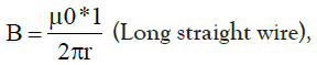
Where I is current, r is the shortest distance to the wire and the constant μo=4π×10−7T m/A is the permeability of free space. (μ0 is one of the basic constants in nature. We will see later that μ ̊ is related to the speed of light.) Since the wire is very long, the magnitude of the field depends only on the distance from the wire ‘r’, not on the position along the wire.

Boundary conditions:

1. Heat transfer in solid

i. Axial symmetry

ii. Heat flux

q₀ = h(T_ext-T)Convective heat flux

Where, h=Heat transfer coefficient

= 20W / (m²k)

T_ext = External Temperature

=293.15[K]

q₀ = Heat Rate

iii. Surface-to-Ambient Radiation:

By using the study of Frequency-Transient

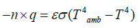
Where, ε = Surface Emissivity

              = 0.1

T_amb = Ambient Temperature

=293.15[K]

2. Magnetic Field (MF):

i. Axial Symmetry

ii. Ampère’s Law

iii. Magnetic Insulation

iv. Coil: Conductor model-homogenized multiturn

Coil excitation-currents

Coil current

No of Turns: N=1

Mesh

Physical-controlled type meshing with normal element size is used (Figure 3).

Figure 3: Meshing

Eement type: Tetrahedrons

Discussion

The simulation has been made to study the temperature and magnetic flux variation for stainless steel, chromium steel, and Iron. The analysis is performed by using different material properties. For a better understanding Figures 4-12 are given below.

Figure 4: Stainless steel magnetic flux.

Figure 5: Stainless steel magnetic flux 3d.

Figure 6: Stainless steel temperature contour.

Figure 7: Chromium steel magnetic flux density.

Figure 8: Chromium steel magnetic flux density (3D).

Figure 9: Chromium steel Temperature contour.

Figure 10: Iron magnet.

Figure 11: Iron Magnetic flux density (3D).

Figure 12: Iron temperature contour.

The comparison between the Magnetic flux densities of different materials and Temperature contours of different materials are displayed in the Table 2 below. It clearly indicates that Chromium steel have minimum Magnetic flux density and Stainless steel have the maximum Magnetic flux density. Also, Stainless Steel has the maximum Temperature contour and Chromium steel have minimum temperature contour.

Table 2: Magnetic flux density and temperature contours.

Conclusion

The numerical study and simulations have been carried out on different materials i.e. stainless steel, chromium steel and iron by using induction heating. In present work the comparative study of temperature and Magnetic flux density distribution done on present materials. The Frequency-Transient study is used to compute temperature changes over time together with the electromagnetic field distribution in the frequency domain. From the results it is observed that stainless steel gives maximum temperature (831.03 K) and Chromium steel gives maximum magnetic flux density (0.04×10^-3).

References

1. Barba PD, Dughiero F, Sieni E. field synthesis for the optimal treatment planning in magnetic fluid     hyperthermia. Arch Electr Eng. 2012;61(1):57-67.

   [Crossref] [Google scholar]

2. Egan LR, Furlani EP. A computer simulation of an induction heating system. IEEE Trans Magn. 1991;27(5): 4343-54.

   [Crossref] [Google scholar]

3. Kozlov AN, Svishchev DA, Donskoy I. Thermal analysis in numerical thermodynamic modeling of solid fuel conversion. J Therm Anal Calorim.2012;109(13):11-13.

   [Crossref] [Google Scholar]

4. Chen M, Dongxu O, Cao S, Jiahao L, Zhi W et al. Effects of heat treatment and SOC on fire behaviors of    lithium-ion batteries pack. J Therm Anal Calorim. 2019;136(6):2429-37.

   [Crossref] [Google Scholar]

5. Chhanwal N, Anishaparvin A, Indrani D, Raghavarao K, Anandharamakrishnan C. Computational fluid dynamics modelling of an electrical heating oven for bread-baking process. J Food Eng.2010;100(3):452-60.

   [Crossref] [Google scholar]

6. Colegrove PA, Shercliff HR. CFD modelling of friction stir welding of thick plate 7449 aluminium alloy. Sci Technol Weld Join. 2006;11(4):429-41.

   [crossref] [Google scholar]

7. Frivaldsky M, Pavelek M, Donic T. Modeling and experimental verification of induction heating of thin molybdenum sheets. Appl Sci. 2021;11(2):647.

   [Crossref] [Google Scholar]

8. Hatou CK, Tchuen G, Woafo P. Modeling, simulation and optimization of solid fuel bread ovens commonly used in developing countries. Heliyon. 2021;7(3):e06585.

   [Crossref] [Google scholar]

9. Muresan C, Achimas G. Fem simulation of medium and large diameter pipe bending using local induction heating. Acta Technica Napocensis. 2014;57(2).[Crossref] [Google scholar]
10. Xiaoming C, Zhe X, Bishi H. Computer simulation of induction heating process of hot rolled slab. Int J Electr Electron Eng Telecommun. 2017;6(4):6-11.

    [Crossref] [Google scholar]

11. Xu, Z, Xuiong C, Bishi, H, Kong Y. Research on temperature optimal control for the continuous casting billet in induction heating process based on ARX Model. Lect Notes Electr Eng.2013;777-786.