Journal of Aeronautics & Aerospace Engineering
Open Access
ISSN: 2168-9792
ISSN: 2168-9792
Research Article - (2018) Volume 7, Issue 1
Three adaptive approaches for a non-linear feed-forward controller are combined with two physics-inspired sinusoidal trajectory planners in a spacecraft attitude control model for large slew maneuvers. The basis of the model is a space based satellite sensor which has suffered an unwanted collision where the inertial matrix of the craft is no longer similar to the originally measured inertial matrix. This causes a large inherent error in the feedforward control needed for system maneuvers due to the mismatch of expected dynamics. Trajectory generation, feedforward control, feedback control, filters, observers, and system stability are discussed in relation to the non-linear dynamics under simulation. The adaptive feed-forward controllers discussed include a proportional-derivative (PD) adaptive controller, a Recursive Least Square (RLS) Method, and an Extended Least Squares (ELS) Method. Mean control effort stayed relatively constant between configurations. The controller configuration with ELS feedforward, PID feed-back, and an extended sinusoidal trajectory outperformed the baseline adaptive controller. Mean error was decreased by 23.4%, error standard deviation by 34.0%, and maximum error by 33.0% from a similar case using RLS adaptation. This improvement is entirely based on a need to correct for un-modeled or mis-modeled dynamics. This scenario occurs in actual operation during spacecraft launch, collisions with debris, or can be caused by fuel slosh or loose components.
Keywords: Adaptation; Satellites; Feedforward Control; Optimal Estimator; Trajectory Planning
A space-based sensor is used to collect many types of data, more specifically there are numerous uses for sensors with high pointing accuracy. The U.S. Department of Defence (DoD) touts the need for highly precise space-based tracking sensors in some recent DoD articles such as studied in [1,2]. They go on to state that this is one of key elements to the modernization of the military’s missile defence strategy. Tracking an object from space requires a small error tolerance. As an example, an arc-minute error from an average low-earth orbiting sensor at an altitude of 800 km [3] can translate to a physical tracking error over 230 meters. When tracking an object much smaller than the size of a football field the object can easily be lost within this error by the space based tracker. Couple the need for precise pointing with the threat of colliding with space debris and other space objects, the possibility of mechanical shifting and settling during a space launch, or the potential mechanical failure, then there is a potential risk of something happening during the life of the sensor such that the physically designed characteristics are no longer as what was designed.
The governing equations for a rotating body such as a satellite are the highly non-linear Newton-Euler equations [4]. Rotation about each major axis affects the others due to cross coupled terms in the mass moment of inertia and cross products of angular velocity. A simple feedback controller is not robust enough against disturbances, or noise, to achieve continuous sub arcminute level performance for attitude control, especially when a fraction of a degree of error causes a vital sensor to be far off-target. Therefore, the full architecture of a non-linear controller is suitable to perform accurate and efficient attitude control at the sub arcminute performance level.
This paper presents a series of simulations using Matlab’s Simulink of a model representative of an actual satellite to include limiting factors such as the control moment gyroscopes (CMGs). The general architecture of the non-linear control approach is discussed first in nonlinear control architecture. In this section three versions of quarter wave sinusoidal trajectories of a constant period are generated and a baseline trajectory is introduced as the base of comparison.
An arbitrarily tough maneuver of a 30° yaw motion was selected to in order to highlight performance differences between the control schemes.
From here the three feedforward control schemes are presented. Feedforward adaptation using proportional-derivative (PD), Recursive Least Square (RLS), and Extended Least Squares (ELS) are presented next. From here a modified PID feedback controller, an Enhanced Luenberger Observer, and a Kalman Filter are presented to complete the description of the overarching simulation. The last component, and arguably most important, to be presented is the route that was taken to show stability in the system. It was decided that showing stability through the use of phase portraits was a necessary first step which is illustrated in results and discussion.
The methodology section presents the methodology of the simulations under test. It goes on to then illustrates the simulation assumptions and limitations. From here the paper then jumps into the results of the simulation experiments in results and discussion which visualize the key benefit of this study: The comparison of the “optimal” RLS error estimator to the ELS error estimator developed in this paper. To perform this unique contribution a progression of six simulations for each trajectory plan are stepped through starting with the results of the feed-forward controller using PD adaptation, then the RLS optimal estimator, then to the ELS estimator. Each case is performed once using a standard proportional-integral-derivative (PID) controller, and then the modified PID controller presented in non-linear control architecture. The phase portrait for the case with the minimum of maximum error is presented in results and discussion. It will be shown that a progressive benefit will arise from implementing a RLS error estimator over PD adaption, and then another increase in performance will be seen by using an ELS estimator over an RLS optimal estimator.
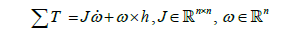
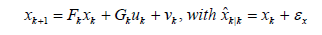
The simulated satellite controller is designed to take input from the user, in this case a 30° change in yaw (ψ), and perform a safe and stable maneuver. First, a trajectory generator converts the user stepinput to a physically possible maneuver. A physics-based feed-forward controller [5] calculates the precise control required to perform the desired maneuver. A feedback controller handles unmodeled dynamics, disturbances, and small discontinuities in the trajectory. The dynamics block shown in Figure 1 represents the actual system and its response to disturbances and inputs. For this research, the governing Newton-Euler equation, shown in Eq. (1), is implemented within the dynamics block and simulated using MATLAB’s Simulink.
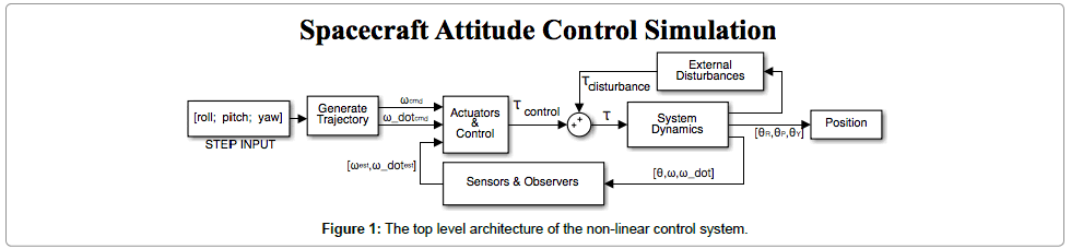
Figure 1: The top level architecture of the non-linear control system.
 (1)
(1)
A disturbance block represents external inputs to the dynamics such as gravity gradient torques due to a centre of gravity offset. Finally, sensors are used to measure the state of the system and filters are used to smooth out the sensor noise. This smoothed data is utilized by the feedback controller and any implemented adaptation in the feed forward controllers. The top-level system architecture of Figure 1 shows the arrangement of the aforementioned components.
Trajectory planning
The first task of this controller is to convert a step-input from the user into an achievable trajectory. Given a desired final state and known initial state, many possible trajectories may be found. One item of note is an additional limitation involved in the trajectory planning is of the CMGs within the simulation. This limitation represents a physical limitation by physical hardware in the control system. If the commanded control torque is too high, then the CMGs will reach their operational limit and the system will not react as expected. This issue is illustrated within the feedback control shown in Section 6. Two methods for trajectory generation were implemented and compared for this controller, both utilizing sinusoidal functions to smoothly rotate to the desired attitudes. The initial method uses a quarter cycle sine function for θ, and the function’s derivative and second derivatives for ω and  respectively. However, this results in discontinuities in the angular velocity and angular acceleration trajectories displayed in Figure 2 in red, which is a 5 second maneuver.
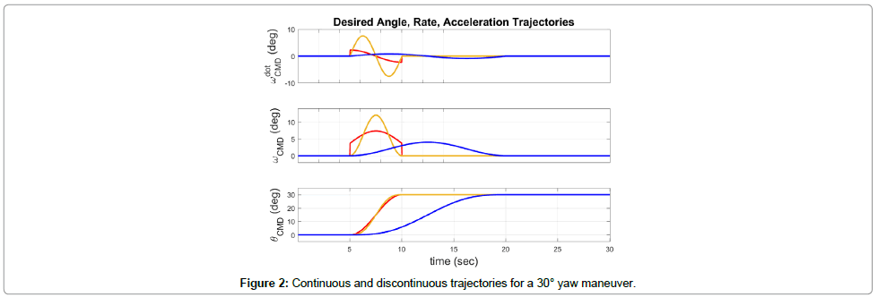
Figure 2: Continuous and discontinuous trajectories for a 30° yaw maneuver.
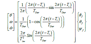
An alternative trajectory was found which is continuous for angular acceleration, and continuously differentiable for angular velocity and position. The closed form equation for a maneuver beginning at time Ti and of duration TDur from a zero state to a desired final state, [φf, θf, ψf ]T, is shown in Eq. (2) and plotted in yellow (a 5 second maneuver) and in blue (a 15 second maneuver) in Figure 2.
 (2)
(2)
Because the angular velocity is zero at the beginning and end of the maneuvers and is continuous during the maneuver, the trajectory is fully achievable given sufficient actuators. The maximum acceleration required can be scaled by changing TDur, the duration of the maneuver. These generated trajectories for, ω, and are passed to the feedforward controller.
Feed forward control
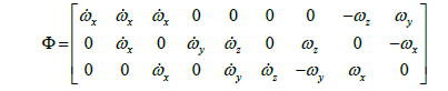
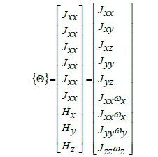
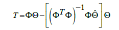
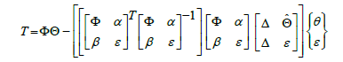
The next task is to select an appropriate feedforward control scheme. The feedforward controller converts the desired trajectories to the corresponding torque inputs for the system actuators. This is achieved by using the non-linear dynamics of the system as described as T= [Φ] {Θ} [6,7] in Eqs. (3) to (5) showcasing the coupling of cross terms and is the matrix representation of the system dynamics which propagates the commanded trajectory as a torque command in the corresponding moment in time.
PD adaptation
Equation (3) represents the original feed-forward control equation presented by Slotine [8], Fossen [9], Sands [10], Byeon [6], and Lavretski [ 11] for control in an idealized system. In this instance the “adaptation” is gained by using an internal feedback loop using a PD control scheme from error between the commanded  and ωd. This idealized approach performs well when the full dynamics of the system are identified and no outside disturbances are felt. However, if this is not the case, then an adaptive feedforward approach should be taken.
 (3)
(3)
 (4)
(4)
 (5)
(5)
RLS adaptation
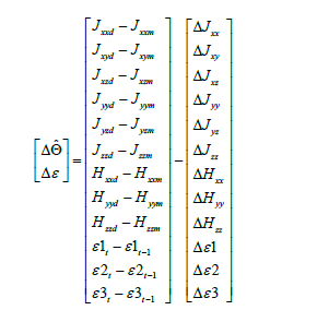
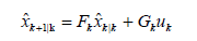
This research utilizes the Recursive Least Squares (RLS) [12,13] and Extended Least Squares (ELS) [14] methodology to achieve adaptation based on the error between the commanded trajectory and the output trajectory of the system dynamics block as shown in Figures 3 and 4 with the assumption of perfect full state feedback. RLS error adaptation is based on the traditional optimal estimator bounded by the brackets within Eq. (6). The expected increased performance in adaptation is due to the fact that the error between commanded and measured angular acceleration and velocity values are propagated forward using the predicted dynamics of the plant to estimate the error in the next time step. The best “fit” in the least squares sense is then estimated.
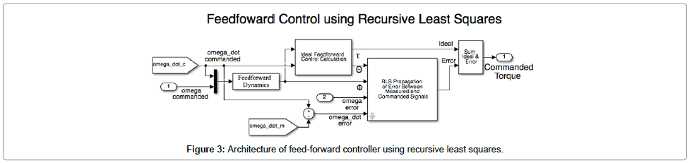
Figure 3: Architecture of feed-forward controller using recursive least squares.
 (6)
(6)
ELS adaptation
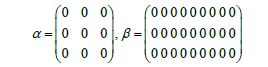
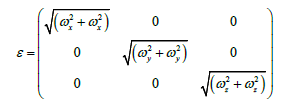
Another method for adaptation in the feed forward controller extends the implementation of RLS from the original RLS implementation in Eqs. (6) and (7) by adding α, β and ε to the original Φ matrix. This creates the feed forward model as seen in Figure 4. Furthermore, the vector is extended as seen in Eq. (8) by adding several extra terms in the adaptive algorithm. The extra degrees of freedom introduced by ε via Eq. (10) does not directly change the adaptation pattern but allow for extra degrees of freedom to establish a best fit in the least squares sense in order to converge more quickly to values of  in Eq. (8). In the specific case of this research, and are sub-matrices of zeros as seen in Eq. (9).

Figure 4: Architecture of feed-forward controller using extended recursive least squares.
 (7)
(7)
 (8)
(8)
 (9)
(9)
 (10)
(10)
Feedback control
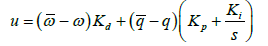
When unmodeled system dynamics are present or when the generated trajectory is unachievable, feedback control is required to eliminate the resulting error [15,16]. An unachievable trajectory can be caused by commanding a high magnitude or discontinuous control signal that overdrives the actuators, CMGs, or thrusters of a space vehicle. A traditional feedback controller may not be able to handle a non-linear plant such as a Van der Pol oscillator as shown in controlling chaos forced van der pol equation [17] but when coupled with a wellfunctioning feed-forward controller a linear feedback controller can suffice. A well-functioning feed-forward controller removes the significant nonlinearities from the system and allows a linear feedback controller to increase the control authority of the system. The modified PID feedback controller shown in Figure 5 uses the error between the ideal trajectory and the observed angular rates and positions to calculate the necessary control. The controller makes use of the full-state feedback from the observers and filters to avoid differentiating a noisy signal [18]. This allows the derivative gain to be much higher than traditional PID controller. The equation for the controller output is shown in Eq. (11).
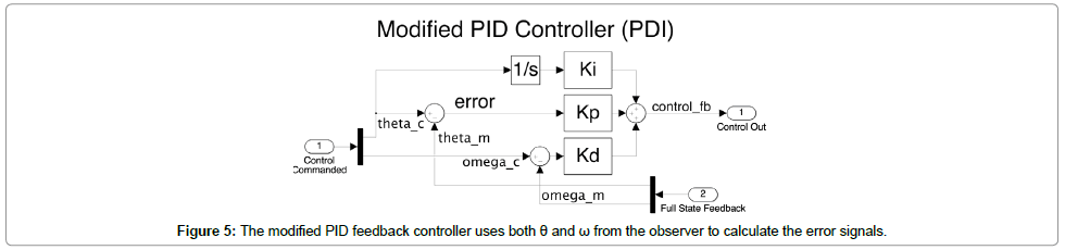
Figure 5: The modified PID feedback controller uses both θ and ω from the observer to calculate the error signals.
 (11)
(11)
Observer design
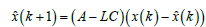
Feedback controllers require a measurement of the actual state of the system [19]. Without noise one can just use a copy of the original system to form full state feedback but an observer is used to calculate the angular accelerations, rates, and positions given the input of a noisy sensor [20]. Equation (12) expresses the general state-space form of a discretized Luenberger observer [21]. Note that in Eqs. (12) and (13), x(k)= {θ (k), ω (k)T}
 (12)
(12)
The Luenberger Observer architecture uses proportional, derivative, and integral gains represented by L (similar to a PID controller) to minimize the error between the measured and calculated angular positions [5]. To avoid differentiating a noisy signal, the “derivative” signal is evaluated by dividing the angular momentum,  , by the moment of inertia, Jp as in Figure 6. is based on the PI observer loop and is akin to the prediction step in a Kalman filter [18] and when the total control signal is fed in to this inner loop it forms an ideal prediction step and reduces observer lag as stated in the state space representation in Eq. (13). This method can allow for better observer performance when dealing with non-linearities.
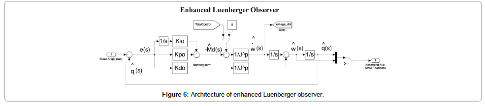
Figure 6: Architecture of enhanced Luenberger observer.
 (13)
(13)
Filter design
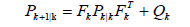
A Kalman Filter is implemented to smooth the measurements found through direct full-state feedback or from the Enhanced Luenberger Observer. The Kalman Filter (KF) [22] in this system is an optimal recursive estimator which uses an identity matrix to represent system dynamics, effectively tracking the system states only through sensor updates. The KF can traditionally be described as an algorithm with two steps: predict and correct [23,24]. The filter is implemented using Eqs. (14) and (18).
Prediction steps
 (14)
(14)
 (15)
(15)
Update steps
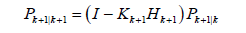
 (16)
(16)
 (17)
(17)
Kalman gain equation
 (18)
(18)
Stability
The most important property of a control system is that it stabilizes the desired system. If the system and controller are unstable, then no other attribute will hold any meaning as the system spins out of control. It is typical to use Lyapunov’s work to prove that a system is stable [25,26]. His work can be broken up into two different methods to prove stability; the indirect and direct methods [27]. For the case where the direct method has no solution an additional concept is introduced, Barbalat’s Lemma [5]. Barbalat’s lemma is called to help show asymptotic stability of a time-varying system. It makes the assumption that if f(t) is differentiable with a finite limit as time goes to infinity, and if f_(t) is continuous, then f_(t) goes to zero as time goes to infinity. We will discuss the indirect method (Figures 7 and 8) [28]. For a non-linear system such as the rotating spacecraft, system stability can be proven by linearizing the system around all points of interest. If the system is stable in these localized regions of interest, then the system is proven stable in a finite range near the equilibrium points [9,28]. For a nonlinear system with many points of interest about which to linearize, this method may be unreasonable. The next viable option in this indirect method of proving stability is through the use of phase portraits. Phase portraits visually represent the relationship between the output and its derivative. In a stable system this representation will show that there exists some finite boundary that all points in the representation will fit into. Figure 9 in the results section shows a phase portrait the final test case scenario. This shows the relationship between θ and ω relative to the yaw control from a representative selection of initial conditions which illustrates the stability of the system as it settles.

Figure 7: Tracking error in yaw position.
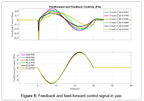
Figure 8: Feedback and feed-forward control signal in yaw.
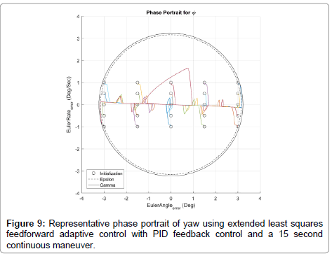
Figure 9: Representative phase portrait of yaw using extended least squares feedforward adaptive control with PID feedback control and a 15 second continuous maneuver.
The goal in this research is to take the Spacecraft Attitude Control model with predetermined system characteristics and improve the performance by modifying some of the functional areas. The two main components chosen to be modified include the trajectory planning and the feedforward sections. Each test case required the feedback controller gains to be manipulated manually to find the best performance in each of the simulation scenarios. The baseline tests utilize the adaptive feedforward control scheme as presented by Slotine [28] using both a PID feedback controller and the modified PDI feedback controller [ 18] using a discontinuous trajectory planner. A continuous trajectory planner was implemented to determine if the prior discontinuities caused worse performance. The RLS and ELS feedforward adaptation methods were implemented to investigate if an improvement can be made over the baseline. Both PID and “PDI” feedback controllers were compared against in each feedforward test case. Considering the different variations there are 12 total variations split fewer than three test cases: Slotine adaptive control, RLS adaptive control, and ELS adaptive control.
The following list presents assumptions made to run MATLAB’s Simulink simulations along with some limitations to the results of the simulations.
Simulation assumptions
1. Sample time is of finite length.
2. No noise was injected into the system during simulations.
3. Gravity gradient disturbances were introduced.
4. The estimated system dynamics in feedforward controller are close enough to actual dynamics for the system to recover.
5. Full-state feedback is given directly to the feedback controllers.
Simulation limitations
1. The system dynamics are calculated with respect to the body frame and not the rotated frame, so errors will grow as the time step increases and causes a perpetual error in the dynamics for the system to adapt to.
2. Feed forward control only functions when a trajectory is currently being pushed to it, otherwise the feedforward control block implements no additional control command.
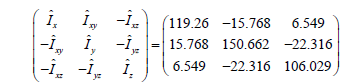
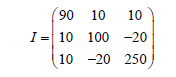
3. The estimated inertial matrix as seen in Eq. (19) is not equal to the true inertial matrix as shown in Eq. (20) which forces the adaptation algorithm to be used.
4. The feedforward control relies upon 9 parameters to be estimated, but the input signal is only comprised of one sine wave. Thus, the algorithm is not experiencing enough excitation for full system identification. These results in the adaptive algorithm to only estimate the parameters that are needed to find the best feedforward control and not the true parameters in the inertial matrix in Eq. (20).
 (19)
(19)
 (20)
(20)
Twelve separate cases were simulated to show the differences between the adaptive control presented by Slotine [28], the use of a recursive least squares algorithm based on some theorems in least squares [12], which utilized statistical digital signal processing and modeling [13]. Additionally, an implementation of the extended least squares algorithm to adapt the feedforward control to miss-modeled dynamics was molded and evaluated. The two different trajectory planners were also compared.
Upon seeing the first simulation runs using the adaptive feedforward control described by Slotine [28], it seemed difficult to find an area to improve. But, as shown in Figure 7, improved performance was possible. Due to the interest in space, Figures 7 and 8 illustrate only the simulations under the continuous trajectory defined in Section 4 and only displays the yaw angle. Similar results were obtained using a discontinuous trajectory but the magnitudes of scale were greater which can be seen in Table 1.
| Variables | Mean-Error | STD Error | Max Error | Mean-Control |
|---|---|---|---|---|
| Base-PID | 0.69546° | 1.3422° | 3.686° | 2.418 Nm |
| RLS-PID | 0.15596° | 0.2591° | 0.379° | 2.819 Nm |
| ELS-PID | 0.29760° | 0.5508° | 1.729° | 2.781 Nm |
| Base-PDI | 0.43338° | 0.8761° | 2.794° | 12.60 Nm |
| RLS-PDI | 0.36381° | 0.9318° | 2.973° | 3.685 Nm |
| ELS-PDI | 0.32679° | 1.1735° | 3.432° | 3.109 Nm |
Table 1: Table comparing simulations results of six control scenarios using a 5 sec discontinuous trajectory.
Additionally, all cases proved to only allow for a small variance in error under the roll and pitch commands which are primarily due to the cross-coupling terms in the system dynamics Equation 2. These errors were negligible when compared to the error in yaw angle and generally converged to zero when the error in yaw converged to zero. Table 2 will show the best results using a continuous trajectory spread across 15 seconds. The test case using ELS Feedforward control with a PID feedback controller shows the smallest standard deviation in error from the commanded trajectory. This can also be seen as the black line in Figure 7. It is interesting to note that all cases using a PID controller outperformed the cases using the modified PDI controller. This is likely due to the exclusion of sensor noise in the simulations.
| Variables | Mean-Error | STD Error | Max Error | Mean-Control |
|---|---|---|---|---|
| Base-PID | 0.0033441° | 0.01059° | -0.0258° | 0.33372 Nm |
| RLS-PID | -0.002019° | 0.00885° | -0.0205° | 0.33395 Nm |
| ELS-PID | -0.002560° | 0.00699° | -0.0173° | 0.33384 Nm |
| Base-PDI | 0.0014662° | 0.02613° | 0.05764° | 0.33189 Nm |
| RLS-PDI | 0.0010740° | 0.02239° | 0.04943° | 0.33384 Nm |
| ELS-PDI | -6.93e-05° | 0.01492° | 0.03193° | 0.33352 Nm |
Table 3: Table comparing simulations results of six control scenarios using a 15 sec continuous trajectory.
To prove stability, simulations were run for initial condition combinations of  Selected simulations of the best controller tested (ERLS-PDI) are plotted in Figure 9. All of the simulations run within the range tested followed the same trends as those shown in the Figure 9. The controlled system is stable. For all initial conditions within ε (a magnitude of 3:1), the state and derivative are zero as t →∞ and never exceed (a magnitude of 3:2).
The ELS-PID controller configuration with the 15 second continuous trajectory had the highest performance. Compared to the recursive least squares optimal error estimator, mean error was decreased by 23.4%, error standard deviation by 34.0%, and max error with reduced by 33.0%. Mean control effort stayed relatively constant. The control effort for all trials was similar mostly due to the extended simulation time averaging out the control.
Stability for other selected cases
As a comparison, additional phase portraits were made for the baseline controller (discontinuous 5-second trajectory, ELS feedforward, PID feedback) and for an intermediate controller (continuous 15-second trajectory, ELS feed forward, PDI feedback). Simulations were run for initial condition combinations of 
Selected simulations of the baseline controller are plotted in Figure 10. All simulations run within the range shown followed the same trends as those plotted below. The controlled system is shown to be stable as, for all initial conditions within ε (a magnitude of 3:1), the state and derivative are zero as t → ∞ and never exceed (a magnitude of 9:6). Selected simulations of the intermediate controller are plotted in Figure 11.
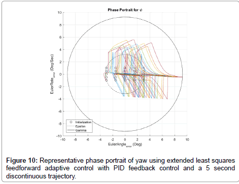
Figure 10: Representative phase portrait of yaw using extended least squares feedforward adaptive control with PID feedback control and a 5 second discontinuous trajectory.
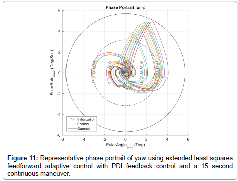
Figure 11: Representative phase portrait of yaw using extended least squares feedforward adaptive control with PDI feedback control and a 15 second continuous maneuver.
All simulations run within the range shown followed the same trends as those plotted below. The controlled system is shown to be stable as, for all initial conditions within " (a magnitude of 3:1), the state and derivative are zero as t → ∞ and never exceed a magnitude of 9.6.
The authors would like to thank Col. Timothy Sands (Ph.D.) for his instructions and assistance in understanding the architecture of non-linear control.
The views expressed in this paper are those of the authors, and do not reflect the official policy or position of the United States Air Force, Department of Defense, or U.S. Government.