The definition of deconvolution is a filtering process that removes a wavelet from the recorded seismic trace [1] and is this done by reversing the process of convolution [2]. The commonest ways that perform deconvolution, by designing a Wiener filter to transform one wavelet into another wavelet in a least-squares sense [3]. It is often applied at least once to marine seismic data. The attenuation of short-period multiples (most notably reverberations from relatively flat, shallow water-bottom) can be achieved with predictive deconvolution [4]. The periodicity of the multiples is exploited to design an operator, which identifies and removes the predictable part of the wavelet, leaving only its non-predictable part (signal) [5].

Algorithm principle

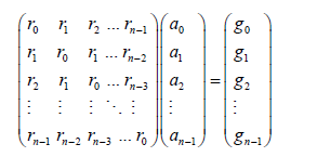
The spiking deconvolution in seismic data processing is routinely applied to compress the source wavelet included in the seismic traces to improve temporal resolution. The general form of the matrix equation for a filter of length n is represented in equation (1), [6]:

(1)

Here, r_i,, a_i, and g_i, i=0,1,2,…..n-1are the autocorrelation lags of the input wavelet, Winer coefficients, and the Crosscorrelation lags of the desired output with the input wavelet respectively.

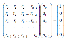
If the desired output is zero delay spike, it is call spiking deconvolution(equation 2):

(2)

The Equation (2) was scaled by (1/ x₀). The least squares inverse filter has the same form as the matrix in equation (2). Therefore, spiking deconvolution is mathematically identical to least squares inverse filter. A distinction, however, is made in practice between the two types of filtering. The autocorrelation matrix on the left side of equation (2) is computed from the input seismogram, in the case of spiking deconvolution (statistical deconvolution), whereas it is computed directly from the known source wavelet in case of least squares inverse filtering. If the input wavelet is not a minimum phase, spiking deconvolution cannot convert it to a perfect zero-lag spike. Although the amplitude spectrum is virtually flat, the phase spectrum of the output is not a minimum phase. The spiking deconvolution operator is the inverse of the minimum-phase equivalent of the input wavelet. This wavelet may or may not be minimum phase.

There is always noise in the seismogram and its additive in both time and frequency domain. An artificial level of white noise is introduced before deconvolution [7]. This is called prewhitening.

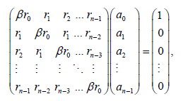
If the percent prewhitening is given by a scalar, 0 ≤ ε < 1, then the normal equations (2) are modified as in equation (3):

(3)

where β = 1 + ε. Adding a constant εr0 to the zero lag of the autocorrelation function is the same as adding white noise to the spectrum, with its total energy equal to that constant.

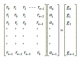
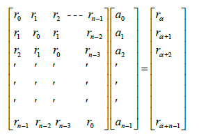
The predicative deconvolution desired output, a time –advance from of input series suggests a predication processes. Given input x (t), we want to predict its value at some full time (t+α), where α is predication lag [8-12]. Wiener show that the filter used to estimate (x+α) can be computed by using a special form of the matrix equation (4) [6].

(4)

Where Here r_i, a_i, and g_i, i=0, 1, 2 ….n, n-1 are the autocorrelation lags of the input wavelet, the Wiener filter coefficients, and the cross correlation lags of the desired output .with the input wavelet respectively. Since the desired output x (t+α) is the time-advance version of the input x (t), we need to specialize the right side of equation (4) for the predication problem. Consider a Five-point input time series x (t): (x₀, x₁, x₂, x₃, x₄), and set α=2. The designed may be carried out using equation (5) and applied on input series as shown in Figure 1.

Figure 1: A flowchart for predictive -deconvolution using predictive filter (Yilmaz [16]).

(5)

Work method

This Process is executed by following steps; first we are going to apply spiking deconvolution. CMP sort is required. For Design window, is entry trace, operator length (240, 128, 40, 10) ms, the percent prewhitening (0%, 1%) for each value of n. Also using amplitude scaling (Mean scale) with applying signal band pass filter (Low Truncation Frequency 10 HZ, Low Cut Frequency 15 HZ, High Cut Frequency 200, High Truncation Frequency 250 HZ). Figure 2 shows the flow were used. The execution parameters, shot _sequence number (0-1856), receiver _sequence _ number (0-59423), channel _number (1-40), CMP _no (0-7478), inline: 2 Xline: 7479[0-7478], input traces (59424).

Figure 2: Show the flow processes for spiking and predictive deconvolution.

The spiking deconvolution algorithm is applied to original data. Figure 1a and the results are shown in Figures 3 and 4. With different operator lengths. Wiener deconvolution causes boosting in random noise, which is standard since it generally boosts the amplitudes of high frequency noise in the data [13-15]. For this reason, a conventional Wiener deconvolution process is generally followed by a band-pass filter to suppress this boosted high frequency noise. The band pass filter parameters are low truncation frequency is 10 Hz, low cut frequency is 15 Hz, high cut frequency is 200 Hz, and high truncation frequency is 250 Hz.

Figure 3: (a) 2d land PSTM Data, CMP sort, before applying spiking-deconvolution, (b) after applying spiking-Deconvolution with Operator-length 240 ms, (c) after applying spiking Deconvolution with Operator-length 128 ms, (d) after applying spiking-Deconvolution with Operator-length 40 ms, (e) after applying spiking- Deconvolution with Operator length 10 ms and the, percent prewhitening for all value of operator-length (0%).

Figure 4: (a) 2d land final PSTM Data CMP sort, before applying spiking deconvolution, (b) after applying spiking Deconvolution with Operator length 240 ms, (c) after applying spiking Deconvolution with Operator length 128 ms, (d) after applying spiking Deconvolution with Operator length 40 ms, (e) after applying spiking Deconvolution with Operator length 10 ms and the, percent prewhitening for all value of operator length (1%).

Second predictive deconvolution, this step creates a new data set with applied trace by trace predictive, No sort is required. For Design window, is entry trace, operator length (240, 128, 40) ms, the predication lag is unity and equal to (α=0 ms, α=1 ms, α=2 ms) sampling rate, the percent prewhitening (1%). Also using amplitude scaling (Mean scale) with applying signal band pass filter (Low Truncation Frequency 10 Hz, Low Cut Frequency 15 Hz, High Cut Frequency 200 Hz, High Truncation Frequency 250 Hz). Figure 2 show the flow was used.

We also applied predictive -Deconvolution with same parameters and α=2 ms, and due gives exactly same results, we won’t display it.

Comparing the seismic data before and after deconvolution, we can see that the deconvolved seismic data shows a significant improvement in vertical resolution and enhanced reflections which correspond to the geology. Such high resolution reflection detail is a desirable feature for seismic interpretation [16,17]. This example indicates that suitable parameters can properly enhance the resolution of the seismic data.

There are many papers done this kind of work but each of them just only took one parameter, or used for other kind of geophysics methods such as Multichannel Wiener deconvolution of vertical seismic profiles [18] and predictive deconvolution in seismic data processing in Atala prospect of rivers State, Nigeria [5]. The second paper was used same methods as in this paper but didn’t show exactly the effect of predication lag due used only one value.

The spiking-deconvolution operator is the inverse of the (minimum phase) equivalent of the input wavelet. This wavelet may or may not be minimum phase. When the source signature is known a designature process can be applied as an alternative or a complement to this step. In our cause we had a different approach. First we applied a trace by trace spiking deconvolution, and the Deconvolution which In this case desired output (zero-lag spike). We tested operator length with n= operator length (where n=240, 128, 40, 20, 10) ms, and the percent prewhitening (1%). Then we test effect of operator length and lags for predicative deconvolution and we found that for spiking deconvolution when operator length was 10 ms and prewhitening (0%) give perfect results (Figure 3e), and for predicative deconvolution Changing the predication lag doesn’t effect, while applying predictive Deconvolution give better results and no matter the value of α (lag) (Figures 5 and 6). The standard equations are solved for the predictive operator in final comparison for each test was made on our data.

Figure 5: (a) 2d land final PSTM Data CMP sort, before applying predictive- deconvolution, (b) after applying predictive-Deconvolution with Operator-length 240 ms, (c) after applying predictive-Deconvolution with Operator- length 128 ms, (d) after applying predictive-Deconvolution with Operator-length 40 ms, (e) after applying predictive -Deconvolution with Operator-length 10 ms and the, lag for all value of operator-length(α=0 ms), and the percent prewhitening for all value of operator length (1%).

Figure 6: (a) before applying predictive-deconvolution, after applying predictive-Deconvolution with Operator-length 240 ms, (b) after applying predictive- Deconvolution with Operator-length 128 ms, (c) after applying predictive-Deconvolution with Operator-length 40 ms, (d) after applying predictive-Deconvolution with Operator- length 10 ms and the, lag for all value of operator-length (α=1ms), and the percent prewhitening for all value of operator- length (1%). (e) Final pstm, (f) data after applying predictive-Deconvolution.

We thank CREWES Project from University of Calgary for giving out permission to use their raw data.