Journal of Proteomics & Bioinformatics
Open Access

Proteoscanner: A Full Proteomics Data Analysis and Visualization Open-Source Software

Ashraf Eltaher^{* *}Correspondence: Ashraf Eltaher, Department of Basic Research, Children's Cancer Hospital, Cairo, Egypt, Email: ,

Author info »

Introduction

Proteomics and metabolomics play a major rule in biological research and biomarker discovery and represent a key-part in understanding the integrated complex biological systems. However, the analysis of proteomics data presents significant obstacles due to the high dimensionality and complexity of the data. Nevertheless, mass spectrometry-based omics data analysis remains challenging due to the numerous widely available data analysis tools, the absence of unified standardized pipeline, the diversity of the generated data formats/sources as well as the data-dependent processing steps. These facts could lead to some confusion in selecting the most appropriate methods and mechanisms for data processing. A vast amount of software’s and web tools had been developed offering different analysis pipelines and data manipulation solutions, some of which provide a powerful robust pipeline but lack optionality while others offer a variety of analysis methodologies with powerful statistics but the quantity and/or quality of available visualization tools is insufficient. Proteoscanner is a user-friendly platform which allows the user to select from various options available for each pre/post-processing stage and/or compare different methods to reach the desired and most accurate analysis results. In addition, it provides precise statistical tests, vivid downloadable figures with publishable qualities and detailed customization options as well as biological interpretation capabilities, such as functional enrichment, over-representation analysis, gene ontologies and protein-protein interactions.

Mass Spectrometry (MS) is a powerful technique of analysis for both identification and quantification of a variety of analytes. When coupled with gas or liquid chromatographs, mass spectrometers expand analytical capabilities to serve more research applications including proteins which drives MS to be an essential analytical tool in the field of proteomics [1].

Modern proteomics experiments generate a vast array of data, presenting a significant challenge in terms of computation and analysis. In terms of complexity, proteomics data is almost>40 times more complex when compared to genomics data of the same test sample, this is due to the huge number of proteins available in comparison to the number of known genes. To address this challenge, sophisticated computational tools are indispensable for distilling these complex datasets into meaningful information. A plethora of attempts to introduce analysis tools that overcome the burdens were done and some great tool solutions were produced. Some of these tools are web-based which have the limitation of the permanent necessity of a powerful internet connection. Other tools are scripting tools which require a prior knowledge of coding and programming languages. Graphical User Interface (GUI) tools are usually user-friendly, but unfortunately, despite being very robust and high quality tools they are, in most cases, either a license-based paid tools or lack accessibility to source code which encounters some flexibility and interoperability issues.

Proteoscanner emerges as a critical solution, specifically designed to streamline the manipulation and analysis of LC/MS-based quantitative proteomics data. The software is an installable, majorly offline-based, free and open source GUI tool. It boasts a wide-scale platform that, although primarily intended for LC/MS proteomic data analysis, offers the versatility to extend to other omics types. This software stands out for its accessibility to users without prior knowledge in programming or statistics, making it a valuable tool for the broader scientific community. Offered as a downloadable package, Proteoscanner includes executable installation and application files along with comprehensive guides and dependencies to ensure ease of use.

In terms of its architecture, Proteoscanner is equipped to handle not only LC/MS-based quantitative proteomics data but also other omics datasets to a certain extent. It incorporates various R packages for analytical functions and utilizes the pyQt5 module for its user interface, enhancing the user experience with a thoughtfully designed dashboard [1].

The database integration of Proteoscanner is extensive, featuring connections with UniProt for protein information retrieval, gProfiler for gene ontology and pathways data from diverse sources and Search Tool for the Retrieval of Interacting Genes/ Proteins (STRING) for constructing networks of protein-protein interactions. Such integration underscores the software's capability in providing a comprehensive suite for biological data interpretation [2-4].

Data loading is designed to be intuitive, offering various options to accommodate different data formats and sources, from local data frames in common file formats to data outputs from established proteomics identification tools. Proteoscanner ensures that the quality of data is verified through a 'Quality check' function before proceeding, laying the groundwork for accurate statistical interpretation.

Proteoscanner's preprocessing panel offers an array of tools for data manipulation and preparation, addressing key steps such as normalization, filtration, imputation and transformation or scaling. These steps are critical for ensuring the integrity and comparability of data within proteomic, metabolomics and transcriptomic datasets. The software does not prescribe a single method but instead a bunch of different techniques, allowing analysts to select the most appropriate method based on the specifics of their data.

The data analysis component of Proteoscanner is built to handle the complexity of omics data, offering both descriptive and inferential statistical approaches. Recommendations for suitable statistical tests are provided based on the nature and distribution of the data and the biological context of the samples.

Visualization capabilities within Proteoscanner are robust and user-customizable, featuring a suite of 19 different graph plots that allow for both pre- and post-processing visualization, ensuring that users can gain comprehensive insights into their data with publishable quality outputs.

Lastly, functional enrichment analysis is another key feature, tapping into biological pathways’ databases to provide deep biological information on the functions and interactions of biological entities.

In summary, Proteoscanner is a multifaceted, user-friendly software designed to meet the diverse needs of the proteomics research community. It provides an integrated solution for data loading, preprocessing, statistical analysis and biological interpretation, all within a single platform. Its open architecture and comprehensive feature set make it an indispensable tool for researchers navigating the complexities of proteomics data.

Materials and Methods

Proteoscanner is a wide-scale software platform designed mainly-but not exclusively for Liquid Chromatography-Mass Spectrometry (LC/MS) proteomic data analysis where it can be extended to other omics types. No prior knowledge of programming or statistics is required-although preferable- as it is appropriate for non-scientific users as well. It is provided as a downloadable package containing an executable installation and application files in addition to installation guide and other dependency files. It is available as an open source tool for windows-based operating systems. Prerequisites for installation are windows 10 or higher as an operating system in which the latest version of both python (python 3.12 at the time of publication) and R (R-4.3.2) is installed. A documentation file for the software is also provided. Figure 1 illustrates the available dashboards and the workflow of Proteoscanner from data uploading towards data manipulation, analysis and visualization down to biological investigation (Figure 2).

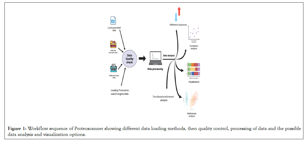
Figure 1: Workflow sequence of Proteoscanner showing different data loading methods, then quality control, processing of data and the possible data analysis and visualization options.

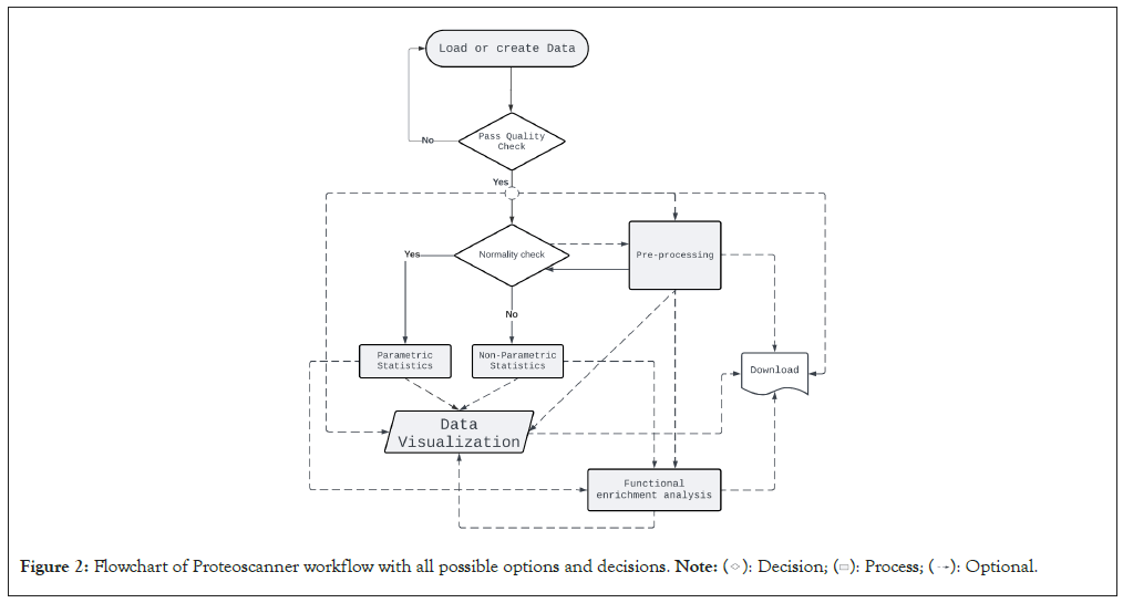
Figure 2: Flowchart of Proteoscanner workflow with all possible options and decisions.

The software is designed to deal mainly with LC/MS based quantitative proteomics data but it is valid partially to any other omics data. Several R packages are used in the analysis functions and the software dashboard was built using the python module pyQt5 graphical user interface designer. Example data integrated within the software to demonstrate its functionality are generated from real datasets obtained from in-house studies inside our laboratory and visualization is facilitated by the ggplot2 package in R, among other specialized packages [5-7].

Results

User interface

Proteoscanner provides a nice, simple and user-friendly interface which drives the user smoothly through the analysis workflow by the help of its six main panels (Figure 3).

Figure 3: Proteoscanner user interface denoted with the six main panels.

Panel 1 for loading data.

Panel 2 for data preprocessing and preparation.

Panel 3 for data statistical analysis and visualizations.

Panel 4 for functional biological interpretation.

Panel 5 for displaying different datasets throughout the session.

Panel 6 for displaying generated figures.

Databases

Uniprot: Used for retrieval of protein information (name and length e.g., in case of Normalized Spectral Abundance Factor (NSAF) calculation in protein pilot software data).

gProfiler: Used for retrieval of gene ontology and pathways information from different sources (Gene ontology, Kyoto Encyclopedia of Genes and Genomes (KEGG), Reactome, Wiki pathways) [8-11].

STRING: Used to generate a network of protein-protein interactions.

Data loading

Proteoscanner offers a user-friendly interface for seamless data loading and management.

Loading of data to Proteoscanner dashboard is available in a variety of options:

Load a local collected data-frame of multiple samples in several formats (csv, txt, xls, xlsx, pkl or RData).

Load a ready available example data.

Load a user-designed data-frame (manual or automatic filling).

Load an output data from several quantitative proteomics identification tools such as Protein Pilot, Peptide Shaker, Proteome Discoverer, MaxQuant or any other tool [12-15].

The loaded data-frame must have a fixed layout (Samples in columns and variables in rows except the first row which should contain the group labels) (Table 1). The id column could be of any known database identifier type or even omics entity names.

Table 1: Proteoscanner loaded data-frame correct layout.

The quality of the uploaded data must be checked first by ‘Quality check’ functionality before proceeding to further steps to ensure its validity for statistical interpretations. Qualified data is the one which is totally numeric (except for the first ID column) and fulfills the layout criteria mentioned above in addition to absence of non-numeric characters or a complete missing column or row.

Data preprocessing

The data processing panel in Proteoscanner provides a comprehensive set of tools to preprocess and edit proteomics data.

There are four main steps of data manipulation and preparation commonly utilized in the pipeline of proteomics along with metabolomics and transcriptomics datasets analysis.

Normalization

The primary aim of normalizing data is to unify the scale for a fair and proper comparison i.e., minimize the technical variations as possible while keeping biological variations.

Quantitative proteomics comparative studies depend primarily on accurate normalization, for which there are a massive variety of choices. Which is the best is based mainly on several criteria such as data type and distribution, Number of samples and the nature of observed values. Some Bioconductor R packages such as limma, Deseq2 and EdgeR are already available and widely used in genomic data normalization and differential analysis but indeed they are not recommended in other types of omics data due to the fact of high dispersibility of genomic data that usually follows negative binomial distribution which is actually not the case in other omics. However, Proteoscanner offers no single recommendation for a normalization method and the decision is left to the analyst to choose from eleven different techniques according to his personal preference which may be-sometimes-affected by the nature of the used data.

Total Sum Normalization (TSN): Normalize each peak in a sample through dividing by the sample’s total peaks [16].

Median Normalization (MN): Normalize each peak in a sample through dividing by the median quotient which is the exponential of the natural logs of all samples’ medians after subtracting their mean from them [17].

Probabilistic Quotient Normalization (PQN): Involves using the highest sample in terms of peaks as a reference sample. The normalization takes place by dividing each peak by the median of its division by the median of the reference sample. [18].

Internal Standard Normalization (ISN): Each peak value is normalized against a selected reference feature where it is divided by the corresponding reference feature value [16].

External Standard Normalization (ESN): Similar to ISN but differs in the reference feature being an external Quality Control (QC) feature of known concentrations in each sample [16].

Compositional Data Approach Normalization (CODA): Data is Centered log-ratio (clr) transformed and its means are calculated then back-transformed to the compositional space using the inverse clr transformation where back-transformed means are used as a scaler denominator for normalization [19].

Robust linear regression normalization (Rlr): This method assumes a linear relationship between the bias in the data and the magnitude of peaks. It fits a linear model by robust regression using an M estimator by Iterated Re-Weighted Least Squares (IWLS). Three variants of Rlr were explored called Rlr, RlrMA and RlrMA cyclic [20,21].

Local regression normalization (Loess): This methods-in contrast to Rlr- assumes a nonlinear relationship between bias and peaks magnitude in which data is first MA transformed then undergoes loess normalization either against the reference average sample (loessF) or pair-wise among all the samples (loessCyc) [21,22].

Variance Stabilization Normalization (VSN): Involves bringing the samples’ variance onto a same scale with a set of parametric transformations and maximum likelihood estimation [17,21].

Quantile Normalization (QN): Involves replacing each sample peak with the mean of the corresponding quantile to force the sample distribution to similarity [21,23].

Eigen MS normalization: This algorithm uses singular value decomposition to capture and remove biases from LC-MS peak intensity measurements. It has the advantage of handling the widespread missing measurements that are typical in LC-MS and has an overfitting-preventing approach. It is suitable to proteomics data [24].

Filtration

Filtering data is a very important aspect which greatly impacts the statistical analysis results. The inclusion of noise, inaccurate or unconfident features should be avoided in order to increase accuracy and minimize statistical type I error. Three different options available for filtering out datasets either per row/feature or per column/sample; a-filtration based on missing value percentage where the features/samples with a percentage of missing values exceeding the user-defined threshold are removed.

b-filtration based on Relative Standard Deviation (RSD) where the features/samples with higher RSD percentage than the userdefined threshold are removed.

c-filtration based on Interquartile Range (IQR) where values which lie outside the IQR of the feature/sample are considered as outliers and removed.

Imputation

In order to go further for differential analysis or statistics, missing values inside the dataset-if any- must be imputed i.e., replaced by real values which should be chosen precisely not to affect the overall data distribution and statistics. User can choose from a variety of commonly-used imputation techniques in omics according to the nature of his data and experimental conditions.

Lowest of Detection methods (LOD): Imputation takes place by using the lowest detected peak value across all the sample or a ratio of it [25].

Left-censored Normal Distribution (lcND): In this approach, missing values are imputed using a random very low value from the data distribution with a mean equal to data mean minus 2.2 standard deviations and a standard deviation of almost third that of the original data.

where X is a random variable with mean=x_μ-2.2x_σ and standard deviation=0.3x_σ, where x_μ, x_σ are original data mean and standard deviation respectively [25].

Hot-Deck Imputation (HD): It is a method in which each missing value is replaced with available values from the same matrix (the donor) [26,27].

k-Nearest Neighbors imputation (kNN): This method imputes missing values in a dataset based on the values of its nearest neighbors [25,27].

Local Least Squares imputation (LLS): It is a local least squares regression model where first, k variables are selected by pearson, spearman or kendall correlation coefficients, then missing values are imputed by a linear combination of the k selected variables [25,28,29].

Random Forest imputation (RF): Better used in the case of mixed-type data. It uses a random forest trained on the observed values of a data matrix to predict the missing values [25,30].

Singular Value Decomposition imputation (SVD): It depends mainly on performing Principal Component Analysis (PCA) for the dataset. Imputation is based on the low-rank approximation obtained from the SVD of the dataset [25,29].

Bayesian Principal Component Analysis imputation (BPCA): Same as SVD but with different mechanism where it incorporates a statistical Bayesian approach allowing for uncertainty estimation [25,29].

Median imputation approaches: Including imputation with the feature median or a random value around with a range of 1% above or below (Median +/- 1%).

Transformation or scaling

Changing the scale or the range of the dataset usually aids in better visualization of data and better inspection of its real distribution. Transformation is-however- somehow more invasive to the dataset than scaling because it results in some alterations in data distribution, intra-distances and betweeness. Therefore, caution should be regarded when transforming data in order not to disturb the real variations or introduce some bias. Selecting the proper scaling method is mostly important for the choice of the suitable statistical test as well as helping for more informative plots. Proteoscanner offers users variable data scaling/transformation mechanisms where they can choose interchangeably among them or either compare with each other. Should the dataset be scaled or not, depends on several aspects including: data nature and distribution as well as the aim of the study, the statistical test to be held and also the personal preference of the statistician.

These four technique are ordered if used simultaneously. If the user wants to change their order, he can perform a multi-step process in the desired order [31,32].

Data annotation

If the id column contains uniprot IDs, Protein names can be retrieved online at any step from uniprot database using uniprotR library in R through the ‘Retrieve protein names’ functionality in the menu bar. This helps for more informative results and visualizations [33].

Data normality

Before proceeding to statistical data analysis, it is strongly recommended to perform a data normality checking to reveal whether the data distribution follows preset assumptions or a known distribution (assumptions-based) or it is assumptions-free i.e., does not follow a known distribution. This type of test is called data parametricity check, where the data which follows one of the normal distributions is called ‘Parametric’ while if not, is called ‘Non-parametric’. This is a very important step in deriving the choice of the statistical tests which will be applied on the data. There are three well-known statistical tests used for checking the normality of the data; Shapiro Wilk’s, Kolmogorov Smirnov and Anderson Darling tests. Each of which provides a p-value threshold upon which the theory of data normal distribution could be accepted or rejected.

Data analysis

Statistics are the most crucial part of omics data analysis and the selection of the most convenient statistical approach is the cornerstone for biological data investigation. No matter the nature and characteristics of your proteomics dataset, you will probably find a suitable statistical test that correctly fits your experimental goal. Both types of statistics; either descriptive in which complete statistics of the data are provided or inferential including correlation, differential expression and fold change analyses are offered. Each of which is supplied with choice recommendations for the user-whenever possible- depending on data distribution and nature of biological samples.

Differential expression: Finding out the main players distinguishing between two or more different sets of observations or different groups of phenotypes is the ultimate goal of differential analysis which leads to uncovering the underlying biological backgrounds. This set of main players is described by being the most statistically significant entities between the tested groups. A variety of statistical tests commonly used in proteomics and/or metabolomics are provided along with recommendations for the suitability of usage for each and the most suitable one in the current case (Figures 4 and 5).

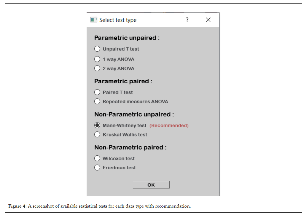
Figure 4: A screenshot of available statistical tests for each data type with recommendation.

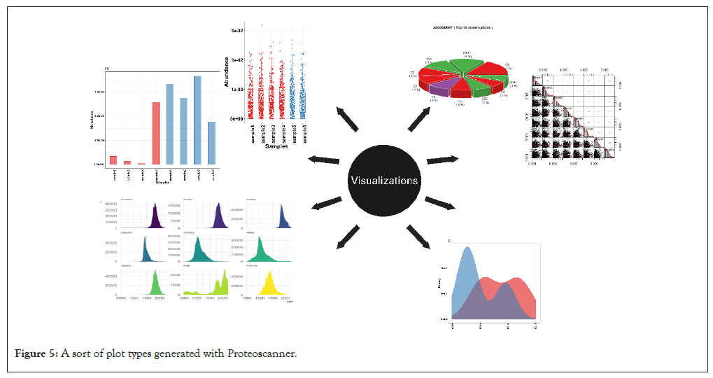
Figure 5: A sort of plot types generated with Proteoscanner.

A significance threshold (p-value or adjusted p-value) is selected also by the user beyond which the statistical difference is significant.

Note: when having more than two groups to be tested, an Analysis of Variance (ANOVA) test is done-or one of its derivatives-followed by a post-hoc test to determine the pairwise differences among the groups (Table 2).

Table 2: Non-parametric Analysis of Variance (ANOVA) with Post-hoc test result.

Correlation analysis: This analysis usually takes place to determine how strong are certain features or samples correlated together so that there is a possible potential biological relationship between them. There are two types of correlation tests (Pearson and Spearman’s correlation). Depending on the data parametricity, we could select either of them. The test results in a correlation coefficient and a p-value for each feature or sample pair. Correlation coefficient ranges from -1 (perfect inverse correlation) to 1 (perfect positive correlation) (Tables 3 and 4).

Table 3: Pair-wise correlation data-frame between samples with p-value.

Table 4: Pair-wise correlation data-frame between samples with p-value.

Fold change analysis: This analysis is valid between two groups only where it calculates the ratio between the two groups’ means in each feature. If more than two groups, user can choose two of them to test. He can choose also how many folds the ratio should be to consider the feature as significantly expressed (Table 4).

Visualization

Effective visualization is crucial for interpreting proteomics data. A very powerful panel of versatile visualization plots is included which provide an outright and comprehensive insights to the data under investigation. The visualization can be held both pre or post-processing. There are 19 different graph plots produced by the help of R packages ggplot2 and others [8,34-46]. You can obtain various flexible, customizable and publishable high-quality graphs which provide an insightful biological image (Figure 5).

Univariate analysis: A collection univariate analysis graphs such as; bar, scatter, line and area plots is included with customization settings to fit different personal preferences. Other figures include heat maps, correlation plots, volcano plots as well as distribution plots (density and box plots).

Multivariate analysis: Proteoscanner contains a panel for the most commonly used multivariate analysis graphs such as PCA, Partial Least Squares-Discriminant Analysis (PLSDA), t-distributed Stochastic Neighbor Embedding (t-SNE) and dendrograms, each of which also contains very detailed customization settings. They are provided with tables of scores and loadings for each feature (table) along with different graphical representations of the analysis results (Figure 6).

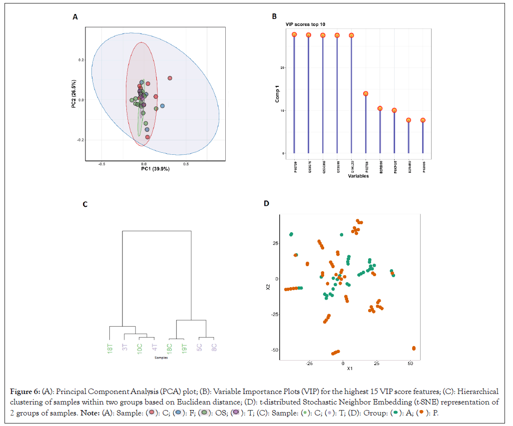
Figure 6: (A): Principal Component Analysis (PCA) plot; (B): Variable Importance Plots (VIP) for the highest 15 VIP score features; (C): Hierarchical clustering of samples within two groups based on Euclidean distance; (D): t-distributed Stochastic Neighbor Embedding (t-SNE) representation of 2 groups of samples.

Networking plots: Networking plots such as; Sankey, chord, pie, donut and network plots show the networking structure and adjacency between entities of choice where the nodes represent the entities and the edges are the connections between them (Figures 7 and 8).

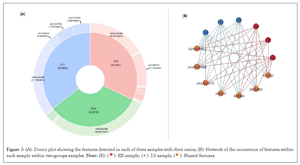
Figure 7: (A): Donut plot showing the features detected in each of three samples with their ratios; (B): Network of the occurrence of features within each sample within two-groups samples.

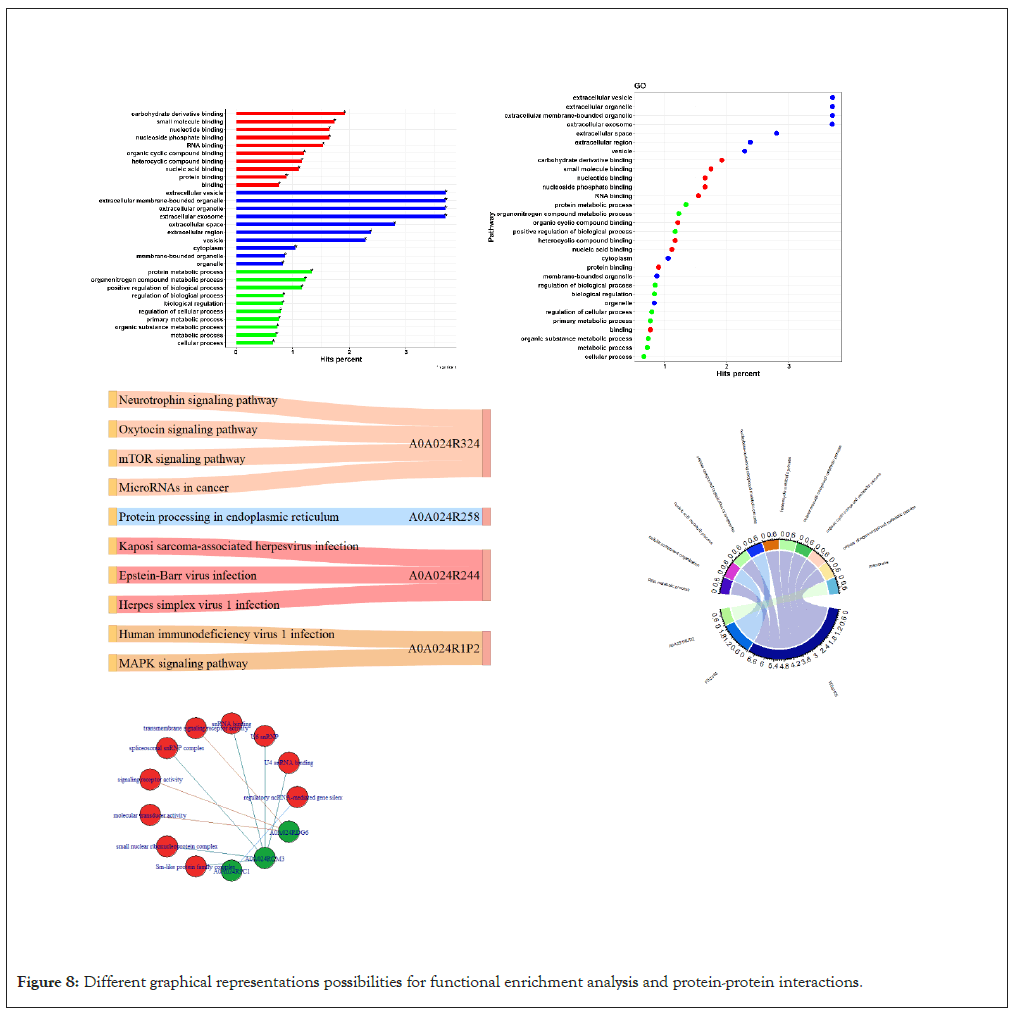
Figure 8: Different graphical representations possibilities for functional enrichment analysis and protein-protein interactions.

Functional enrichment

The biological interpretation is the utmost objective for omics data analysis. Accordingly, biological insights must be inferenced accurately for a biological experiment to be scientifically valid. Functional enrichment analysis provides a profound biological information of the whereabouts and functions of the biological entities. Databases such as KEGG, Reactome and Wiki pathways along with others contain information about biological pathways of different organisms [9-11].

Gene Ontology (GO) database provides a framework and set of concepts for describing the functions of gene products where it supports the computational representation of biological systems. It consists of three major components; biological process, molecular function and cellular component [8].

Over Representation Analysis (ORA) is a statistical method for objectively determining whether a gene set or pathway is more prevalent or relevantly enriched in a set of biological entities such as genes, proteins or metabolites than we expect by chance. This provides an image of the gene ontology components or pathways in which our biological variables of interest are significantly represented.

The software utilizes this method through its biological enrichment functionalities using gprofiler2 package in R (ref) which retain information from the GO, KEGG, Reactome and Wiki pathways databases. The results are displayed both in a table form (table) and also with various visualization possibilities (Figure 8) [7,9-11].

Protein-protein interaction is another functionality for retrieving and displaying information about interactions between proteins of interest both tabular and graphically as a network retrieved from STRING database for protein interactions through STRINGdb library in R [4].

Discussion

Proteoscanner was developed as a standalone open-source software using python and R programming languages. It provides a framework for proteomics -and other omics- data full analysis pipeline with a multi-optional, flexible and user friendly dashboard. Through case studies spanning a diverse set of biological samples, Proteoscanner has demonstrated its robustness and efficacy in generating clear biological insights. These case studies serve to underscore the software’s versatility in handling varying analytical demands and its capacity to deliver meaningful interpretations of biological data. While it offers recommendations for data processing, statistical test selection and visualization based on our team's statistical expertise, it intentionally leaves room for the researcher's discretion due to the absence of a single standardized pipeline for LC/MS proteomics. This flexibility empowers researchers to tailor the analysis to their unique requirements, selecting from a myriad of analytical pathways without constraint.

The dashboard consists of four main tool panels for data loading, data processing/statistical analysis, wealthy visualization plots possibilities and biological functional interpretation. This is in addition to two additional panels for the display of tables and figures. Each panel has a variety of buttons and functionalities to fit for different data formats, analysis approaches and methodologies. Researchers are allowed to apply a single function or a group of functions simultaneously in any order, select from a variety of choices according to their analyzed data type whilst a recommendation to the best choice is also offered. The software is freely available and is an open source platform which is suitable for both researchers and non-scientific individuals.

Conclusion

Proteoscanner is a comprehensive software package that empowers researchers to analyze and interpret proteomics data efficiently and accurately without the need for complicated calculations or exhausting coding. By integrating data loading, data processing, visualization plots and functional enrichment analysis, Proteoscanner provides a user-friendly interface for both novice and expert users. The software offers a range of advanced features and algorithms, enabling researchers to uncover valuable biological insights from complex proteomics experiments. Proteoscanner represents a significant advancement in the field of proteomics data analysis and holds great promise for accelerating discoveries in the field of proteomics research. Moreover, the software is available as an open-source which accounts for more adjustability and continuous improvement.

Acknowledgement

We would like to acknowledge the contributions of the proteomics and metabolomics research unit at children cancer hospital 57357 and everyone who contributed to open-source libraries used in Proteoscanner. We must also enlighten the effort of Renad Alaa and Ala’a Ahmed for participating with their effort and time in the software interface layout refinement and the software materials’ testing. This work would not have been possible without their valuable efforts.

References

1. Willman J. Beginning PyQt - A Hands-on Approach to GUI Programming. Apress. 2020.

   [Crossref]

2. UniProt Consortium. The universal protein resource (UniProt). Nucleic Acids Res. 2007;36:D190-195.

   [Crossref] [Google Scholar] [PubMed]

3. Reimand J, Kull M, Peterson H, Hansen J, Vilo J. g: Profiler-a web-based toolset for functional profiling of gene lists from large-scale experiments. Nucleic Acids Res. 2007;35:W193-200.

   [Crossref] [Google Scholar] [PubMed]

4. Szklarczyk D, Kirsch R, Koutrouli M, Nastou K, Mehryary F, Hachilif R, et al. The STRING database in 2023: protein-protein association networks and functional enrichment analyses for any sequenced genome of interest. Nucleic Acids Res. 2023;51(D1):D638-D646.

   [Crossref] [Google Scholar] [PubMed]

5. Sameh M, Khalaf HM, Anwar AM, Osama A, Ahmed EA, Mahgoub S, et al. Integrated multiomics analysis to infer COVID-19 biological insights. Sci Rep. 2023;13(1):1802.

   [Crossref] [Google Scholar] [PubMed]

6. Alaa M, Al-Shehaby N, Anwar AM, Farid N, Shawky MS, Zamzam M, et al. Comparative Shotgun Proteomics Reveals the Characteristic Protein Signature of Osteosarcoma Subtypes. Cells. 2023;12(17):2179.

   [Crossref] [Google Scholar] [PubMed]

7. Wickham H. ggplot2: Elegant Graphics for Data Analysis. Springer International Publishing. 2016.

   [Google Scholar]

8. Ashburner M, Ball CA, Blake JA, Botstein D, Butler H, Cherry JM, et al. Gene ontology: tool for the unification of biology. Nat Genet. 2000;25(1):25-29.

   [Crossref] [Google Scholar] [PubMed]

9. Kanehisa M, Goto S. KEGG: kyoto encyclopedia of genes and genomes. Nucleic Acids Res. 2000;28(1):27-30.

   [Crossref] [Google Scholar] [PubMed]

10. Croft D, O’kelly G, Wu G, Haw R, Gillespie M, Matthews L, et al. Reactome: a database of reactions, pathways and biological processes. Nucleic Acids Res. 2010;39:D691-697.

    [Crossref] [Google Scholar] [PubMed]

11. Agrawal A, Balcı H, Hanspers K, Coort SL, Martens M, Slenter DN, et al. WikiPathways 2024: next generation pathway database. Nucleic Acids Res. 2024;52(D1):D679-689.

    [Crossref] [Google Scholar] [PubMed]

12. Seymour SL, Hunter CL. ProteinPilot™ Software Overview. High quality, in-depth protein identification and protein expression analysis. 2015.

    [Google Scholar]

13. Farag YM, Horro C, Vaudel M, Barsnes H. PeptideShaker online: a user-friendly web-based framework for the identification of mass spectrometry-based proteomics data. J Proteome Res. 2021;20(12):5419-5423.

    [Crossref] [Google Scholar] [PubMed]

14. Orsburn BC. Proteome discoverer-a community enhanced data processing suite for protein informatics. Proteomes. 2021;9(1):15.

    [Crossref] [Google Scholar] [PubMed]

15. Tyanova S, Temu T, Cox J. The MaxQuant computational platform for mass spectrometry-based shotgun proteomics. Nat Protoc. 2016;11(12):2301-2319.

    [Crossref] [Google Scholar] [PubMed]

16. Noonan MJ, Tinnesand HV, Buesching CD. Normalizing gas-chromatography-mass spectrometry data: method choice can alter biological inference. BioEssays. 2018;40(6):1700210.

    [Crossref] [Google Scholar] [PubMed]

17. Ritchie ME, Phipson B, Wu DI, Hu Y, Law CW, Shi W, et al. limma powers differential expression analyses for RNA-sequencing and microarray studies. Nucleic Acids Res. 2015;43(7):e47.

    [Crossref] [Google Scholar] [PubMed]

18. Gotsmy M, Brunmair J, Büschl C, Gerner C, Zanghellini J. Probabilistic quotient’s work and pharmacokinetics’ contribution: countering size effect in metabolic time series measurements. BMC Bioinformatics. 2022;23(1):379.

    [Crossref] [Google Scholar] [PubMed]

19. Aitchison J. The statistical analysis of compositional data. J R Stat Series B Methodol. 1982;44(2):139-160.

    [Crossref] [Google Scholar]

20. Venables WN, Ripley BD. Modern Applied Statistics with S. Springer, New York. 2002.

    [Crossref] [Google Scholar]

21. Välikangas T, Suomi T, Elo LL. A systematic evaluation of normalization methods in quantitative label-free proteomics. Brief Bioinform. 2018;19(1):1-11.

    [Crossref] [Google Scholar] [PubMed]

22. Willforss J, Chawade A, Levander F. NormalyzerDE: online tool for improved normalization of omics expression data and high-sensitivity differential expression analysis. J Proteome Res. 2018;18(2):732-740.

    [Crossref] [Google Scholar] [PubMed]

23. Bolstad BM. preprocessCore: A collection of pre-processing functions. R package version. 2023;1(0):2.

    [Crossref] [Google Scholar]

24. Karpievitch YV, Nikolic SB, Wilson R, Sharman JE, Edwards LM. Metabolomics data normalization with EigenMS. PloS One. 2014;9(12):e116221.

    [Crossref] [Google Scholar] [PubMed]

25. Jin L, Bi Y, Hu C, Qu J, Shen S, Wang X, et al. A comparative study of evaluating missing value imputation methods in label-free proteomics. Sci Rep. 2021;11(1):1760.

    [Crossref] [Google Scholar] [PubMed]

26. Joenssen DW, Bankhofer U. Hot deck methods for imputing missing data: the effects of limiting donor usage. Machine Learning and Data Mining in Pattern Recognition: 8th International Conference. 2012;7376:63-75.

    [Google Scholar]

27. Kowarik A, Templ M. Imputation with the R Package VIM. J Stat Softw. 2016;74(7):1-6.

    [Crossref] [Google Scholar]

28. Kim H, Golub GH, Park H. Missing value estimation for DNA microarray gene expression data: local least squares imputation. Bioinformatics. 2005;21(2):187-198.

    [Crossref] [Google Scholar] [PubMed]

29. Stacklies W, Redestig H, Scholz M, Walther D, Selbig J. pcaMethods-a bioconductor package providing PCA methods for incomplete data. Bioinformatics. 2007;23(9):1164-1167.

    [Crossref] [Google Scholar] [PubMed]

30. Stekhoven DJ, Bühlmann P. MissForest-non-parametric missing value imputation for mixed-type data. Bioinformatics. 2012;28(1):112-118.

    [Crossref] [Google Scholar] [PubMed]

31. Kucheryavskiy S. mdatools-R package for chemometrics. Chemom Intell Lab Syst. 2020;198:103937.

    [Crossref] [Google Scholar]

32. Murphy K, Viroli C, Gormley IC. Infinite mixtures of infinite factor analysers. Bayesian Anal. 2020;15(3):937-963.

    [Google Scholar]

33. Soudy M, Anwar AM, Ahmed EA, Osama A, Ezzeldin S, Mahgoub S, et al. UniprotR: Retrieving and visualizing protein sequence and functional information from Universal Protein Resource (UniProt knowledgebase). J Proteomics. 2020;213:103613.

    [Crossref] [Google Scholar] [PubMed]

34. Chen H, Boutros PC. VennDiagram: a package for the generation of highly-customizable Venn and Euler diagrams in R. BMC Bioinformatics. 2011;12:35.

    [Crossref] [Google Scholar] [PubMed]

35. Lemon J. Plotrix: a package in the red light district of R. R-news. 2006;6(4):8-12.

    [Google Scholar]

36. Moon K. autoReg: Automatic Linear and Logistic Regression and Survival Analysis. R package version 0.3.4. 2023.
37. Gu Z, Gu L, Eils R, Schlesner M, Brors B. "Circlize" implements and enhances circular visualization in R. Bioinformatics. 2014;30(19):2811-2812.

    [Crossref] [Google Scholar] [PubMed]

38. Kolde R. Pheatmap: pretty heatmaps. R package version. 2019;1(2):726.

    [Google Scholar]

39. Simko T, Wei TR. R package “corrplot”: Visualization of a Correlation Matrix. Version 0.88. 2021.

    [Google Scholar]

40. Peterson BG, Carl P, Boudt K, Bennett R, Ulrich J, Zivot E, et al. PerformanceAnalytics: Econometric tools for performance and risk analysis. R package version. 2014;1(3).

    [Google Scholar]

41. Galili T. dendextend: an R package for visualizing, adjusting and comparing trees of hierarchical clustering. Bioinformatics. 2015;31(22):3718-3720.

    [Crossref] [Google Scholar] [PubMed]

42. Csardi G, Nepusz T. The igraph software package for complex network research. Complex Syst. 2006;1695(5):1-9.

    [Google Scholar]

43. Allaire J, Ellis P, Gandrud C, Kuo K, Lewis B, Owen J, et al. Package ‘networkD3’. D3 JavaScript network graphs from R. 2017.

    [Google Scholar]

44. Kassambara A, Mundt F. Factoextra: extract and visualize the results of multivariate data analyses. R package version 1.0.7. 2020.
45. Kuhn M. Building predictive models in R using the caret package. Journal of statistical software. 2008;28(5):1-26.

    [Crossref] [Google Scholar]

46. John CR, Watson D, Lewis M, Russ D, Goldmann K, Ehrenstein M, et al. M3C: A Monte Carlo reference-based consensus clustering algorithm. Sci Rep. 2018:10(1):1816.

    [Crossref] [Google Scholar] [PubMed]