Journal of Proteomics & Bioinformatics
Open Access
ISSN: 0974-276X
ISSN: 0974-276X
Research Article - (2018) Volume 11, Issue 10
Keywords: Parp-1; GA-MLR; Phthalazinones; Y-randomization
PARP-1 is increasingly gaining attention as an anticancer pharmacological target in both preclinical examinations and clinical trials. In the treatment of breast cancer, ovarian cancer, prostate cancer, pancreatic cancer and unspecified solid tumors, some PARP- 1 inhibitors/antagonist have received FDA approval such as olaparib (AZD2281), veliparib (ABT-888), and rucaparib (AG-014699) [1-4]. Inhibition of PARP-1 results to the accumulation of DNA damage. This occurs by impairing single-strand DNA break repair (SSBR) and trapping PARP-1 at single-strand break sites, which leads to inhibition of DNA replication [4]. The role of PARP-1 includes cell proliferation, survival and death; this is due to its effects on the regulation of multiple biological processes [5,6]. Recent studies have shown that metastasis, deterioration and angiogenesis in tumors are associated with elevated expression of PARP-1 protein [7,8]. The role of PARP-1 in cancer therapy makes it an interesting target for inhibition by small molecules. Recently, a novel series of phthalazinones as inhibitors of PARP-1 have been reported by Loh and colleagues [9]. The experimental estimations of the inhibitory activity of chemical molecules is difficult, timeconsuming and expensive, therefore, a great deal of effort has been required into attempting the measurements of activity via statistical modeling. QSAR analysis is an effective approach in research which has been applied into rational drug design and the mechanism of drug actions. In QSAR studies, biological activities of compounds are expressed as a function of their various structural properties which explains how the variation in biological activity relies on changes in the chemical structures [10]. The advances of QSAR study depends largely on choosing a robust statistical methods for producing the predictive model and also the required structural properties for expressing the essential features within those chemical structures. In recent times, genetic algorithms (GA) are widely adopted methods for variable selection [11-13]. In this study, we report the development of a QSAR model for PARP-1 inhibition which has not yet been done.
Accession of experimental data
In this present Quantitative Structure-Activity Relationship (QSAR) study, a set of twenty-six (26) Phthalazinones was retrieved from the CHEMBL database (http://www.ebi.ac.uk/chembl) with accession ID of CHEMBL1141921 [14]. This dataset represent a novel series of potent inhibitors of poly (ADP-ribose) polymerase in terms of IC50 (μM). The biological activity data (IC50) were then converted to PIC50 values using the formula PIC50= (-Log (IC50 X) (was used as the depended variable). The structures of Phthalazinones are listed in Table 1 with their observed activities.
| S/N | CHEMBL ID | CHEMICAL STRUCTURES | IC50 (nM) | pIC50 (nM) |
Normalized Data (nM) |
| 1 | CHEMBL193917 | 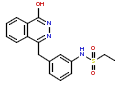 |
290 | 6.54 | 0.189 |
| 2 | CHEMBL383578 | 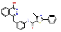 |
27 | 7.57 | 0.64 |
| 3 | CHEMBL66761 | 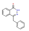 |
770 | 6.11 | 0 |
| 4 | CHEMBL370692 | 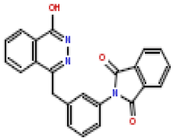 |
180 | 6.75 | 0.281 |
| 5 | CHEMBL196450 |  |
6.8 | 8.17 | 0.904 |
| 6 | CHEMBL193918 |  |
189 | 6.72 | 0.268 |
| 7 | CHEMBL363617 |  |
13 | 7.89 | 0.781 |
| 8 | CHEMBL195913 |  |
19 | 7.72 | 0.706 |
| 9 | CHEMBL196444 |  |
5 | 8.3 | 0.961 |
| 10 | CHEMBL197192 |  |
9.8 | 8.01 | 0.833 |
| 11 | CHEMBL371244 |  |
36 | 7.44 | 0.583 |
| 12 | CHEMBL193512 |  |
370 | 6.43 | 0.14 |
| 13 | CHEMBL195402 |  |
12 | 7.92 | 0.794 |
| 14 | CHEMBL436298 |  |
5 | 8.3 | 0.961 |
| 15 | CHEMBL196507 |  |
55 | 7.26 | 0.504 |
| 16 | CHEMBL371205 |  |
33 | 7.48 | 0.601 |
| 17 | CHEMBL195966 |  |
9.5 | 8.02 | 0.838 |
| 18 | CHEMBL370217 |  |
4.1 | 8.39 | 1 |
| 19 | CHEMBL381652 |  |
90 | 7.05 | 0.412 |
| 20 | CHEMBL425560 |  |
90 | 7.05 | 0.412 |
| 21 | CHEMBL381208 |  |
50 | 7.3 | 0.522 |
| 22 | CHEMBL196559 |  |
120 | 6.92 | 0.355 |
| 23 | CHEMBL371425 |  |
20 | 7.7 | 0.697 |
| 24 | CHEMBL382950 |  |
10 | 8 | 0.829 |
| 25 | CHEMBL193903 |  |
47 | 7.33 | 0.535 |
| 26 | CHEMBL372450 |  |
56 | 7.25 | 0.5 |
Accession of chemical structures
The canonical smiles of Phthalazinones obtained from the CHEMBL database were converted to SDF files with 2D and 3D coordinates using data Warrior software version 4.7.2. The 2D and 3D QSAR model generated in this study was derived from the training dataset of 20 molecules while the predictive potential of this model was evaluated by the test set of 6 molecules with uniformly distributed biological activities. Table 2 shows the observed and predicted biological activities of the training and test datasets.
| Training Set | Selected Descriptors | Observed and Predicted values | Outlier Information | |||
|---|---|---|---|---|---|---|
| Compounds | khs.aasC | bpol | TPSA | Observed | Predicted | Outlier |
| 2 | 1 | 0.793 | 0.219 | 0.64 | 0.523117788 | - |
| 3 | 0 | 0 | 0.231 | 0 | 8.01E-04 | - |
| 4 | 0.667 | 0.399 | 0.519 | 0.281 | 0.704651415 | - |
| 5 | 0.5 | 0.676 | 0.868 | 0.904 | 0.876213482 | - |
| 6 | 0.667 | 0.297 | 0 | 0.268 | 0.174108841 | - |
| 7 | 0.333 | 0.272 | 0.588 | 0.781 | 0.561471385 | - |
| 8 | 0.333 | 0.377 | 0.739 | 0.706 | 0.694655479 | - |
| 9 | 0.333 | 0.423 | 0.939 | 0.961 | 0.897221843 | - |
| 10 | 0.5 | 0.659 | 0.799 | 0.833 | 0.80664574 | - |
| 12 | 0.333 | 0.52 | 0.363 | 0.14 | 0.24932188 | - |
| 13 | 0.167 | 0.416 | 0.898 | 0.794 | 0.729157094 | - |
| 14 | 0.5 | 0.405 | 0.822 | 0.961 | 0.902829557 | - |
| 15 | 0.167 | 0.411 | 0.712 | 0.504 | 0.530150087 | - |
| 16 | 0.333 | 0.654 | 0.882 | 0.601 | 0.770868974 | - |
| 17 | 0.5 | 0.71 | 0.855 | 0.838 | 0.852648456 | - |
| 18 | 0.333 | 0.549 | 1 | 1 | 0.927528838 | - |
| 20 | 0.167 | 0.538 | 0.62 | 0.412 | 0.395320488 | - |
| 22 | 0.167 | 0.487 | 0.587 | 0.355 | 0.374099969 | - |
| 24 | 1 | 1 | 0.489 | 0.829 | 0.755849723 | - |
| 25 | 0.667 | 0.648 | 0.502 | 0.535 | 0.616338063 | - |
| Test set | Selected Descriptors | Observed and Predicted values | AD information | |||
| Compounds | khs.aasC | bpol | TPSA | Observed | Predicted | AD |
| 1 | 0.333 | 0.714 | 0.385 | 0.189 | 0.218491495 | - |
| 11 | 0.167 | 0.294 | 0.947 | 0.583 | 0.816249215 | - |
| 19 | 0.167 | 0.284 | 0.71 | 0.412 | 0.563695923 | - |
| 21 | 0.167 | 0.411 | 0.967 | 0.522 | 0.804909229 | - |
| 23 | 0.167 | 0.411 | 0.824 | 0.697 | 0.650828612 | - |
| 26 | 0.667 | 0.675 | 0.374 | 0.5 | 0.470829812 | - |
Table 2: Normalized values of selected descriptors and the observed/predicted Y values (Normalized values).
Descriptors generation
In order to develop a Quantitative Structure-Activity Relationship (QSAR) model, the biological activity of compounds must be quantitatively represented by molecular descriptors. The Chemistry Development Kit (CDK) descriptor version 1.0 was used for the calculation of different descriptors under the following categories: Topological descriptors, Geometric descriptors, Hybrid descriptors, Electronic descriptors and Constitutional descriptors. The calculated descriptors were arranged in a data matrix. The preprocessing or pretreatment of the independent variables (i.e., descriptors) was done by removing invariable (constant column) and other descriptors based on a variance cut-off of 0.0001 and correlation coefficient cut-off of 0.99 using J Frame VWSP version 1.0.
Data normalization
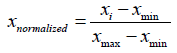
Due to the existence of much variability in the range and distribution of each variable in the data set, the calculated values of the descriptors of each compound with their corresponding biological activity were subjected to a statistical technique known as min-max normalization using Normalize. The Data software version 1.0. In min-max normalization, the minimum and maximum value of each variable is adjusted to a uniform range between 0 and 1 according to the following equation:
 (1)
(1)
Where xnormalized represents the min-max normalized value, xi represents the value of interest, xmin represents the minimum value, and xmax represents the maximum value.
Selection of training and test set
The dataset of 26 Phthalazinones molecules was divided into training and test set based on Kennard-Stone method [15,16] using the J Frame Division software version 1.0. In this method, dissimilarity value gives an idea to handle training and test set size. This method is used for MLR model with pIC50 activity values as dependent variable and the various 2D and 3D descriptors calculated for the molecules as independent variables.
QSAR Model development
In this study, QSAR model was developed from the dataset using the Multiple linear regression (MLR) method to screen potential leads against PARP-1 within a training dataset set (20 compounds). The total molecular descriptors (108) was calculated for each compound using CDK algorithm. Finally, a robust QSAR model equation was derived by MLR; Irrelevant descriptors were removed based on the Inter Correlation cut-off of 0.99 and Variance cut off of 0.001 using the Genetic Algorithm v4.1 software which leads to a selection of three (3) descriptors (one 3D and two 2D) in the final QSAR regression equation (Table 2). The model creates a relationship in the form of a straight line (linear) equation that best approximates all the individual data points. Regression equation takes the form.
Y = b1x1 + b2x2 + b3x3 Equation 2
Where Y is dependent variable, ‘b’s are regression coefficients for corresponding ‘x’s (independent variable), ‘c’ is a regression constant or intercept.
Model validation
Model validation is necessary in QSAR modeling, it confirms the reliability of the developed QSAR model along with the acceptability of each step during model development [17]. Model validation is done to test the internal stability and predictive ability of the QSAR models. The developed QSAR models in this study were validated by the following method:
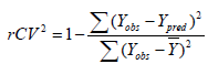
Internal validation: Internal validation was carried out using leave-one-out (LOO-) method. In the leave-one-out (LOO) method of cross validation, the process of removing a molecule, and creating and validating the model against the individual molecules is performed for all the Q2 (rCV2) values and reported. The rCV2 (cross-validation regression coefficient) was calculated using equation (3), which describes the internal stability of a model.
 (3)
(3)
In the above equation, Y-means the average activity value of the training dataset, while Yobs and Ypred represent the observed and predicted activity values respectively. A high rCV (>0.5) suggests a reasonably robust model [18].
Estimation of the predictive ability of a QSAR model: After the internal validation process, the high predictive power of a QSAR model should be estimated from an external test set of compounds that are not used in building of the QSAR model. The external validation or predictive capacity of the obtained model was judged by predictive R2 (Rpred2) as shown in given equation:
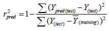 (4)
(4)
Where Ypred (test) and Y(test) indicate the predicted and observed activity values, respectively, for test set compounds and Y(training) indicates the average bioactivity of compound in the training set. An acceptable predictive power of a QSAR model (Rpred2) should be >0.6 for the test set molecules [19-21].
GA-Multiple linear regression
According to the inter-correlation coefficients of the descriptors, highly correlated descriptors were removed from the study by a genetic algorithm method using a correlation regression cut-off of 0.99. According to the rule of thumb in MLR (ratio of sample size to the number of descriptors should be greater than or equal to 5), a tetraparametric model can be expected with the current training set of 20 compounds. This can be shown below:
pIC50 = -0.2481(+/-0.1155) +0.7582(+/-0.2042) khs.aasC -0.2811(+/-0.2448) bpol +1.0775(+/-0.1539) TPSA
n = 20, R2 = 0.8038, R2a = 0.767, F = 21.85072, q2 = 0.6727, r2pred=0.61915, SEE=0.1421, SDEP= 0.1641, PRESS : 0.32297
The above equation indicates that the model obtained with GAMLR showed good squared correlation coefficient (R2) value and good internal predictive power (rCV2) with an excellent external predictive power (r2pred). The scatter plot which is plotted between observed and predicted pIC50 values for training set and test set are shown in the Figure 1a and b respectively. A plot of the residual for the predicted values for both the test and training data sets against the experimental pIC50 values is shown in Figure 2. It can be deduced from the plot that the model did not show any proportional and systematic error. This is because the propagation of the residuals on both sides of the zero are random. The derived QSAR model fitted with GA-MLR presents a significant relationship between pIC50 values (dependent variable) and the selected descriptors (independent variables). The value of the regression coefficient (R2=0.8038) indicates the existence of ~80.4% correlation between the activity and the selected descriptors in the training dataset, while the value of the cross-validation regression coefficient (q2 = 0.6727) suggests ~67.2% prediction accuracy of this QSAR model. This QSAR model fitted with GA-MLR can be use to predict future observations. Rpred2= 0.61915, shows the predictive power of the model. To judge the overall significance of the regression coefficients, the variance ratio (F) is computed. The F value has two degrees of freedom: p, N-p-1. For overall significance of the regression coefficients, the F value should be high. Also, for a good model, the standard error of estimate (SEE) of Y should be low. Finally, model predictivity is judged using the predicted residual sum of squares (PRESS) and cross-validated R2 (Q2) for the model while the value of standard deviation of error of prediction (SDEP) is calculated from PRESS.

Figure 1: GA-MLR analysis showing the correlation between observed and predicted pIC50 values for the (A) Training set and (B) Test set.

Figure 2: Plot of residual versus experimental pIC50.
Y-Randomization
The Y-randomization test was carried out in order to ensure that there is no random correlation. By this, we could validate the established QSAR model and confirm that the selected descriptors are not random, and consequently, the result model should have low statistical quality. Random MLR models are generated in this test. This is done by randomly shuffling the dependent variable while keeping the independent variables as it is. The newly established QSAR models are expected to give significantly low values of R2 and Q2 for several trials; which confirm that the developed QSAR models are robust [22]. In this study, five trials of Y-randomization was carried out and the five random models generated gave lower values of R2 and Q2 thereby validating the original model (the established GA-MLR model) (Table 3). Another parameter; cRp2 is also estimated, which should be greater than 0.5 for passing the test [22] following the equation below:
| Model | R | R2 | Q2 |
|---|---|---|---|
| Original | 0.896552594 | 0.803806554 | 0.672688449 |
| Random 1 | 0.624637279 | 0.39017173 | -0.208879566 |
| Random 2 | 0.439219719 | 0.192913962 | -0.180816154 |
| Random 3 | 0.232298582 | 0.053962631 | -0.556768219 |
| Random 4 | 0.528915084 | 0.279751166 | -0.057761159 |
| Random 5 | 0.48867299 | 0.238801291 | -0.474684813 |
Table 3: Five trials Y-randomization outcome.
cRp2=R*(R2-(Average Rr)2)1/2
Where Rr=Average ‘R’ of random models
Table 4 shows that the cRp2 calculated in this study is 0.688462594 which is greater than 0.5 and thus confirmed that the test is passed.
Applicability domain
Applicability Domain (AD) refers to the response and chemical structure space in which the QSAR model makes predictions with a given reliability [22]. We carried out the AD using standardization approach in order to find out the test set compounds that falls outside the applicability domain and also to detect training set compounds that are outliers. The software adopted for this analysis is called “AD using standardization approach”. This software is developed in java language at Drug Theoretics and Chemoinformatics laboratory. Table 4 reveals that there is no outliers among the training set which conforms with the normal distribution pattern of about 99.7% of the population remaining with the range mean of ± 3 standard deviation (SD). Thus, mean ± 3 describes the region where most of the training data set compounds belong to. Any compound found outside this region is dissimilar to the rest and majority of the compounds. Table 5 also show that no test compound is found outside the AD. Therefore, this suggests that the QSAR model developed in this study can make predictions with a given reliability. Another required aspect is how to evaluate the performance of AD. The rule that is universally accepted is that the prediction error (PE) of the compound inside the AD should be lesser than the compound that are outside the AD [22]. Because all the test set compounds appear in the true positive quadrant, they are said to be inside the applicability domain Figure 3.

Figure 3: Test set compounds within the AD (MDI=Model Disturbance Index).
| Random Models Parameters | |
|---|---|
| Average r : | 0.462748731 |
| Average r^2 : | 0.231120156 |
| Average Q^2 : | -0.295781982 |
| cRp^2 : | 0.688462594 |
Table 4: Y-randomization model’s quality check parameters.
| S/N | Descriptors | Description |
|---|---|---|
| 1 | khs.aasC (2D) | A fragment count descriptor that uses e-state fragments. Traditionally the e-state descriptors identify the relevant fragments and then evaluate the actual e-state value |
| 2 | bpol (2D) | Sum of the absolute value of the difference between atomic polarizabilities of all bonded atoms in the molecule (including implicit hydrogens) |
| 3 | TPSA (3D) | Sum of solvent accessible surface areas of atoms with absolute value of partial charges greater than or equal 0.2 |
Table 5: Selected descriptors with their respective description.
In this study, GA-MLR was used in the construction of a robust QSAR model for Parp-1 inhibitors. Several validation techniques were used to validate the derived model. The model show good predictive potential for Parp-1 inhibitors which can be use to predict new Parp- 1 inhibitors. These QSAR model could provide a reliable tool for the design of Parp-1 inhibitors.