As results of rapid growth in wireless communications, there are more demands for proper network coverage prediction. A good field coverage prediction requires a deep understanding of the limitations caused by environmental condition to the wave propagation. Methods for predicting wave propagation coverage is being developed for decades. These methods predict the path propagation loss at a given point. The propagation models can be classified in to three models: empirical model, stochastic model and deterministic model. Empirical models are those models that based on the observations and measurements alone. These models are mainly used to predict the path loss [1]. Empirical models can be described by equations derived from a statistical analysis of a large number of measurements. The models are doing not require very detailed information about the environment. The input parameters for the empirical models are usually qualitative and not very specific; one of the main drawbacks of empirical models is that they cannot be used for different environments without modification. The okumura model, hata model and cost 231-hata mode are popular empirical models. For the application of the empirical models, some model parameters should be determined for different environments, which are usually done with some optimization techniques. The several empirical models are used to model a suburban area and compared with the experimental data. The results show that measurement data are more close to the Hata model [2]. For the urban coverage, a path loss model is developed with regression fitting method, by which the prediction error can reduced. The model uses linear model and have the limitation for the more complexes propagation path and environments [3]. The Bertoni-Walfisch model is first model which takes into consideration the effect of buildings on radio propagation channel in path-loss modelling [4]. The model assumes that propagation takes place over rows of buildings having equal heights and equal spacing arranged in a perfect grid. Bertoni-Walfisch model has 5 parameters, which is optimized with measurement data. Another empirical model is Davidson model, which is a derivative of the Hata model. The optimization for Davidson model shows that the path loss exponent depends the propagation environments [5]. The effect of land cover is studied and the optimization method improves the standard deviation of the error from 9.6 to 6.3 dB [6]. However, the land cover data are required as input parameters, which have effects to the accuracy of prediction.

In this paper, a stochastic differential method is used to study the wave propagation in the complexed environment. First, the SDE model is constructed for the wave propagation. Then the simulation parameters in the SDE model are explained for the simulation in the complexed environment. The validation of the SDE model is made for averaging 5000 samples of propagation loss curve and compared with the theoretical results. In order to use the SDE method to a specified environment, the parameters in SDE are explained, which can be related to the specified environment. The field measurements in Beijing are performed and the comparisons between the experimental data and SDE simulation results are made and good results are obtained [7].

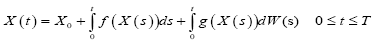
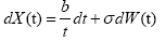
The loss of wave propagation is a function of the environment. For the complex environment, there are many random factors which make the loss prediction more difficult. The traditional approach uses the experimental formula to treat the wave propagation in complexed environment, such as buildings in large city. Stochastic differential equation method has been applied in a range of application areas, including biology, chemistry, epidemiology, mechanics, microelectronics, economics, and finance. Here the SDE is used to predict the propagation loss in the complexed environment and the environment is considered as a random factor. White noise cannot be constructed as an ordinary function of distance, say Z (d). It should be regarded a generalized function, or “distribution” of the type described by Schwartz. Since noise is a generalized function, it must appear inside integration.

(1)

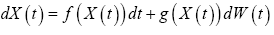
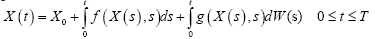
Where X (t) is Stochastic process and for fixed t, X (t) is random variant, W (t) represent Brown motion. Its differential equation is really short hand for an integral equation:

(2)

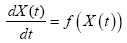
In Equation (2), if function g is zero, stochastic differential equation becomes the ordinary differential equation.

(3)

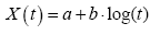
In order to model the wave propagation problem, it is necessary to construct the SDE model for the wave propagation in the complexed building up areas. Firstly, considering the free space propagation, it is well known that the propagation loss is proportional to logarithm of the distance t, that is

(4)

The differential form of the Equation (4) can be written as:

(5)

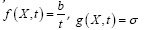
Comparing with differential Equation (3), there is

(6)

In the complexed environment, the SDE is constructed as:

(7)

Here the parameters b describes the average loss in the complexed environment as a distance changes and by gives the variance that is caused the irregularity in propagation path.

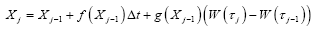
After completing the SDE model construction for wave propagation, the simulations are made to validate the SDE model for the wave propagation. For the numerical simulation of SDE, the dW(t) in the Equation (7) is described as Brownian motion. By Ito integral, the integral form of SDE can be written as:

(8)

Where,

The numerical formula for simulation is

(9)

Validation of the stochastic differential equation model

In order to validate the model that developed in Equation (7), the simulation is made for different propagation loss index b and variance parameter σ. Generally, for wave propagation in free space, the propagation loss index is 2 and for the complexed environment, the propagation loss index will be increased because the obstacles. In the free space case with small fluctuation terrain, here assume b=2, and σ =1. Figure 1a gives the comparison between the theory result and SDE average result of 5000 samples. It is seen that the two results have a good agreement. Further comparison is made to more fluctuation case in which σ =5 as shown in Figure 1b. Due to the large fluctuation, the average of 5000 displays a little discrepancy that can be decrease by increase the sample numbers in average. The samples number of average has a significant effect to the propagation loss as shown in Figure 1c. When the samples number of average is not large enough, the seed of the random generator has also an effect to the propagation loss along the path. The SDE model simulation uses many parameters. The parameters can be related to the practical loss prediction of the wave propagation. In the field measurement, the measurement data is limited, so the measured propagation loss is not regularly. The samples number of average can be used to describe the irregularly propagation loss. The different environment has a different propagation loss, which can be attributed to the seed of random generator.

Figure 1a: Normalized propagation loss. SDE simulation parameterb=2, σ=1, samples number for average 5000.

Figure 1b: Normalized propagation loss. SDE simulation parameter b=2, σ=5, samples number for average 5000.

Figure 1c: Normalized propagation loss. SDE simulation parameter b=2, σ=5, samples number for average 500.

SDE method for loss prediction

In order to study the prediction of propagation loss, a transmitter which broadcasts in 546 MHz and antenna height is 293 m are used for measurement. The EM field polarization is vertical. For measuring the electromagnetic fields, the following equipment are used: an E-field measurement device with a monopole whip antenna, a geolocation finder (GPS) and lastly a laptop computer to be able to record measured results and location information together with them. The measurements are gathered within the range starting from a point which is very close to transmitter and ending at location which is 8 kilometres away from it for Beijing Guomao TV transmitter. The height of the antenna is 197 m. Another measurement is gathered for Beijing Xijiao TV transmitter, in which the height of antenna is 293 m, the test range ends at location 11.2 kilometres away from it. The whip antenna was connected to the measurement device on the top of a vehicle and the location information was recorded automatically simultaneously.

The comparison is made between the Guomao experiment and the SDE prediction as shown in Figure 2. In order to fit the SDE model, the index of propagation loss is selected as b=20, which represent a large propagation loss for this area. Considering there are many higher buildings in this area, the large propagation loss is expected. The variance σ = 6 is chosen, which states the random loss that is caused by the random building distribution. The irregularity of the propagation loss as function of distance can be described by the samples number of average; here samples number is taken as 20 for the average. The different seed of random generator can give different propagation loss curve for finite samples average, which can be used as a selection for predicting loss in different place or different propagation environment. The Figures 2a and 2b use the seed 2 and 99 respectively in matlab random generator. It is show that Figure 2a gives a large prediction loss and Figure 2b gives a small prediction loss relative theory curve. The characteristics of the SDE can be used to model the different type random distributed buildings. By this method, it is reasonable to use the Figure 2a as the predicted propagation loss for the planning purpose.

Figure 2a: Comparison for measurement in Guomao and SDE prediction. The SDE simulation parameters: b=20, σ=6, samples number for average m=20, random generator seed=2.

Figure 2b: Comparison for measurement in Guomao and SDE prediction. The SDE simulation parameters: b=20, σ=6, samples number.

For average m=20, random generator seed=99.

Similar as the above, the comparison is made between the Xijiao experiment and the SDE prediction as shown in Figures 3a and 3b. Compared to Guomao area, the buildings in Xijiao are lower and less crowded than the Guomao’s. From the Figure 3, it is seen that index of propagation loss is b=13, which means the less propagation loss compared with Guomao. The variance is also chosen as 6. The samples number for average is 20. Like the above, the random generator seed 2 can give a large loss and seed 99 give a small loss. So it is reasonable to use the Figure 3a as the predicted propagation loss for the Xijiao area.

Figure 3a: Comparison for measurement in XiJiao and SDE prediction. The SDE simulation parameters: b=13, σ=6, samples number for average m=20, random generator seed=2.

Figure 3b: Comparison for measurement in XiJiao and SDE prediction. The SDE simulation parameters: b=13, σ =6, samples number for average m=20, random generator seed=99.

The loss of wave propagation is affected by many factors in the complexed environment such large city and mountain area. Because the random of the environment, the loss of propagation has the different characteristics in different area, which make the accreted prediction loss difficulty. The stochastic differential equation method is used in a range of application areas, including biology, chemistry, epidemiology, mechanics, microelectronics, economics, and finance. In this paper the SDE method is used to predict the wave propagation loss. Firstly, the SDE model is constructed for the wave propagation, which is validated by comparing the SDE result and theoretical result. Then, the meaning of the SDE parameters is explained, in which parameter b is respond to the index of median propagation loss, the variance σ for the random distribution of the propagation environment, the samples number of average for the irregularity of loss along the path, the seed of random generator for the specified propagation environment.

The SDE method is used to analyse the experiment data that are performed in two areas of Beijing. The building in Guomao area is more crowed and higher than the Xijiao area. The measured data shows a large loss in Guomao than Xijiao. The index parameter b of SDE model indicates that b is 20 for the Guomao and 13 for the Xijiao, which is reasonable. In order to describe the irregularity along the distance, the sample number of average is taken as 20. The seed of random generator is 2 in matlab function rng, which is more close to the measurement result.

To sum up, the SDE method presents us a new method to study the wave propagation. The parameters of SDE model are given the meaning to explain the loss of wave propagation in the complexed environment, which will be helpful for the planning purpose.