Journal of Stock & Forex Trading
Open Access

Simulation Study of Foreign Exchange Market Interventions using an Extended Dealer Model

Rintaro Arita, Hideki Takayasu and Misako Takayasu^{* *}Correspondence: Misako Takayasu, Department of Computing, Tokyo Institute of Technology, Tokyo, Japan, Email:

Author info »

Introduction

Financial market research is conducted in various fields such as economics, financial engineering and econophysics, clarifying various properties of financial markets [1-10]. In recent years, algorithmic traders known as High Frequency Traders (HFT) have been participating in financial markets, rapidly placing and canceling orders, thus significantly impacting the market [11-13]. Data in financial markets can be classified into three types such as macroscopic, mesoscopic and microscopic. Macroscopic data consist of time series of price fluctuations, revealing various statistical properties of price time series such as the power law of volatility [14-18]. Mesoscopic data refers to order book data, analyzing and modeling the properties of order book behind price movements [19-21]. Microscopic data refers to the behavioral data of individual dealers participating in the financial market and models exist that focus on the behavior of various dealers [22-29]. These models belong to a type of agent-based model, where multiple agents follow certain rules to generate artificial markets.

The dealer model proposed by Takayasu et al., is a pioneering model of the agent-based models [25]. By modeling the investment strategies of dealers, the Dealer Model (DM) artificially generates financial markets and enables analyzing the mechanism of price formation. The model incorporates the effect of anticipating future price movements based on past price fluctuations. Exact solutions for the two-body dealer model were derived, revealing the relationship between dealers’ trend-following effect and the power-law behavior of volatility and approximate solutions for the multi-body dealer model were derived using the mean-field approximation theory, replicates most of the empirical statistical properties in the market.

While the dealer model successfully reproduced most statistical properties of stable markets, additional effects are necessary to replicate the properties of unstable markets. A typical example of an unstable market is the market during FX intervention. FX intervention refers to actions taken by monetary authorities in the foreign exchange market to influence exchange rates, often referred to as foreign exchange market interventions. In Japan, a large-scale dollar-bought (yen-sold) intervention occurred in 2011. Additionally, in 2022, the Bank of Japan conducted dollar-sold (yen-bought) interventions to halt excessive yen depreciation, in contrast to the intervention in 2011. FX interventions have been analyzed in the field of economics, studying their methods and effects [30-35].

To simulate the unstable market conditions during interventions, the dealer model was enhanced as follows [36]. Since the entire order book widens during large price movements, the effect of the dealer’s spread widening as volatility increase was introduced into the dealer model. Additionally, the effects of FX interventions, dealer’s stop-loss and take-profit behaviors were incorporated. Particularly, the distinctive price movements during the 2011 intervention could be partially replicated using this improved model.

This article was first analysed not only the price movements but also the order book data during the interventions in 2011 and 2022. It revealed that interventions in 2022 were conducted with significantly different strategies compared to those in 2011. To replicate the market conditions during these interventions, it further improved the dealer model to conduct simulations closer to real-market scenarios. Furthermore, by conducting a parameter search of the dealer model, it developed a systematic simulation method to reproduce the market conditions during interventions. In this study, data from the USD/JPY foreign exchange market on the EBS Data Mine Level 2.0 was used.

Materials and Methods

Real data analysis

In order to investigate the impact of order size and price increments on trade execution and price discovery over time, comparing the 2011 and 2022 datasets. Some real data analysis was performed as given below:

Electronic Broking Services (EBS) FX data: Electronic Broking Services (EBS) is a market for interbank trading in foreign exchange, where a large amount of transactions take place. In the USD/JPY foreign exchange market, the minimum order size is 1 million USD and trading volumes range from approximately 10 to 20 billion USD per day. The data consists of order book and transaction data, recorded every 100 milliseconds. The order book data includes the order prices, quantities and bid or ask status for the top 10 orders at each timestamp, starting from the best order. The minimum size for order prices is 0.001 yen in the 2011 data and 0.005 yen in the 2022 data. Transaction data includes the transaction price, quantity, timestamp of the transaction and whether the transaction was executed by selling or buying.

FX intervention: To influence the FX market, central banks sometimes intervene in the market, which is known as foreign exchange intervention. For example, in Japan, to prevent excessive depreciation of the yen, the Bank of Japan conducted interventions by selling dollars and buying yen. Specifically, on 21st October, 2011, interventions amounted to approximately 8.1 trillion yen, while on 21st October, 2022, interventions amounted to approximately 5.6 trillion yen [37].

Figures 1a and 1b, are the market price time series on 21st October, 2011 and 21st October, 2022, respectively, showing significant price fluctuations. Figure 1, show the shape of the order book before and during interventions in 2011 and 2022, respectively (Figure 1).

During the intervention in 2011, as shown in Figure 1(i), there were orders within approximately 10 levels in the order book. However, during the intervention in Figure 1(ii), it can be observed that there were over 16,000 bids at 79.2 yen. This indicates that a large number of bids were placed as if building a wall to keep the price constant. In the intervention of 2022, as shown in Figure 1(iii), there were orders within approximately 10 levels in the order book. However, during the intervention in Figure 1(iv), it can be observed that there were around 40 asks priced more than 1 yen below the best bid. This suggests an intervention aimed at significantly lowering the price by placing asks below the best bid.

Figure 1: Rate time series of USD/JPY at the particular time. a) 21 October, 2011; b) 21 October, 2022; (i-iv) The shape of the order book at the mentioned time on Figures 1a and 1b.

Extension of the dealer model

Basic dealer model: The dealer model focuses on the behavior of dealers participating in the market, proposed by Takayasu et al., in 1992 [25]. The dealer model is known as a model capable of artificially reproducing financial markets. Subsequently, the dealer model was formulated as a probabilistic model and it was demonstrated that various statistical properties observed in the market, such as the power-law behavior of volatility and the distribution of transaction time intervals, can be reproduced.

In the dealer model, it is assumed that each dealer participating in the market holds one ask and one bid, denoted as a_i(t) and b_i(t), respectively. The difference between a_i(t) and b_i(t) is referred to as the spread and denoted as s_i(t), while the average of a_i(t) and b_i(t) is denoted as p_i(t). Thus, a_i(t) and b_i(t) can be expressed in terms of p_i(t) and s_i(t) as follows.

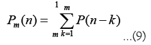
The stochastic dealer model is formulated as follows.

P(n) denotes the market price at the n^th tick. A tick is a unit of time that increments by 1 for each transaction. ⟨ΔP⟩_m is the weighted average of price differences over the past m ticks, corresponding to the trend-following effect. For dealers with d_i>0, if the price has recently increased, they anticipate further increases and adjust their order prices upwards. For dealers with d_i<0, if they anticipate that recent price changes will not continue, they adjust their order prices in the opposite direction of recent price changes. The third term is a noise term, taking ΔP with probability 1/2 and -ΔP with probability 1/2.

Figure 2, depicts a schematic diagram of the dealer model for the case of two dealers. Figures 2a and 2b, shows that based on equation 3, dealers adjust their order prices. Figure 2c, shows that a trade occurs when the ask and bid prices of dealer’s match, i.e., when min_i a_i(t) ≤ maxi b_i(t). Figure 2d, shows that trading occurs at P(n)=(min a_i(t)+max b_i(t))/2 and the dealer who traded returns the mid-price p_i(t) to P(n). Then, the process returns to (a) (Figure 2).

Figure 2: Schematic diagram of the dealer model. A) Schematic diagram of the dealer model for N=2; B) Diagram of the dealer model with volume effects. Dealers hold multiple orders and when orders match, trades are executed based on the number of orders from the dealer with the lower order quantity. Note: (a,b) The trend-following random walk with Equation 3; (c) If the best ask ≤ best bid, a trade is conducted; (d) The dealer who conducted the trade in c returns their order price pi to the transaction price P(n) and returns to a.

Spread dealer model: Matsunaga et al., proposed the spread dealer model as a model capable of reproducing the unstable state of markets during events such as the Lehman Shock or FX interventions [36]. In the spread dealer model, when the volatility |∆P| is high, the spread of dealers widens. Additionally, to reproduce the price changes during interventions, the effects of stop-loss and take-profit actions, as well as intervention effects, were added. The spread dealer model is expressed as follows.

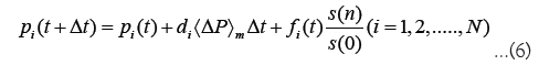
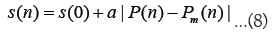
For simplicity, it is assumed that the spread s_i is the same for all dealers. By adding this effect, the correlation between the distance of the centers of gravity of the ask and bid and volatility observed in the real market can be well approximated. The term (s(n)/s(0)) in equation 6 adjusts the noise term according to changes in the spread, aiming to keep the trend-following effect constant by adjusting the dealer’s jump width to maintain a constant distribution of trading time intervals.

Furthermore, by calculating the dealer’s position and computing the profit and loss PL_i(n), the effects of stop-loss and take-profit were added. Stop-loss occurs when the dealer’s loss exceeds a certain amount, i.e., when PL_i(n)<PL_lc, leading to the resolution of the position to realize the loss. Take-profit occurs when a profit of Rp has been achieved from the profit and loss x ticks ago, i.e., when PL_i(n)<R_p. PL(n-x), leading to the resolution of the position to realize the profit.

In addition, the following two types of intervention effects were introduced.

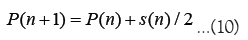
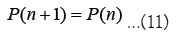
Equation 10 corresponds to market order intervention, the effect is to increase the market price by half the spread Equation 11 corresponds to limit order intervention, it is added as the effect of keeping the market price constant.

Extended spread dealer model: The spread dealer model successfully reproduced the price fluctuations during interventions in 2011 and the correlation between the spread and volatility. However, it simulated price movements over a short tick time, which is not consistent with the number of ticks and trading volume observed in the market during the intervention. To simulate price fluctuations aligned with the observed number of ticks during interventions, this study introduced volume into the spread dealer model, modified the intervention effects, adjusted the stop-loss and take-profit effects and formulated them.

Firstly, to introduce the concept of volume into the dealer model, dealers are assumed to randomly place multiple orders in the market. When orders match, they are executed according to the number of orders from the dealer with fewer orders, while orders from the dealer with more orders remain in the market. If all of the orders are executed, the dealer places multiple orders randomly again.

Next, modifications were made to the intervention effects. In addition to normal dealers, an intervention dealer performing the following intervention actions was introduced.

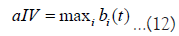
These intervention dealers do not usually participate in trading but perform one of the intervention actions at a certain time. Equations 12 and 13 correspond to market orders, where the intervention dealer offers the best price. Equation 14 corresponds to building a limit order wall, where the intervention dealer continues to place buy orders for 79.2 yen. Equation 15 corresponds to intervention with limit orders placed at a price γ yen lower than the best bid. For example, γ=1.15. These interventions are assumed to occur with a certain probability p_iv and if intervention occurs volumes, the intervention dealer withdraws from the market.

Furthermore, the stop-loss and take-profit effects are modified and formulated as follows. The dealer’s valuation profit and loss PL_i(n) is calculated and if PL_i(n) exceeds a certain threshold, the dealer will execute a stop-loss or take-profit action with a certain probability plc(ptp). Specifically, if PL_i(n)<PL_lc or PL_i(n)>PL_tp.

PL_i(n) is calculated using Equation 17, as the tick increases with each trade, based on the dealer’s current position Pos_i(n) and the total value of positions at the time of trading B_i(n).

Pos_i(n) and B_i(n) are determined as follows when v volume of trades are executed where dealer i’s ask and dealer j’s bid match at price P.

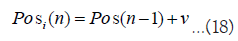
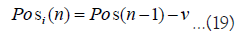
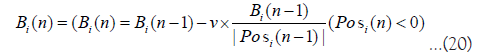
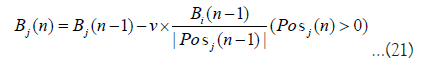
Pos_i(n) increases or decreases by the number of executed orders. B_i(n) increases by the purchase price when adding to the position and decreases by the price per position when partially closing the position.

Additionally, a profit-taking dealer is introduced as an initial condition with a certain position. If positions are skewed to one side, due to intervention, take-profit will not occur. To prevent this, a profit-taking dealer who holds a certain number of positions as an initial condition was introduced.

Results

Reproduction of the basic statistical properties observed in the market

The basic statistical properties observed in the market can be reproduced by a dealer model that introduces volume. Figure 3, presents a comparison of statistical properties between the real market and the dealer model. The parameters used in the simulation are shown in (Table 1). From Figure 3a, it can be seen that the power law behavior of volatility |∆P| observed in the real market is reproduced. From Figure 3b, it can be seen that the autocorrelation function R(k) of the price difference ∆P, takes a negative value at the first tick, as observed in the real market (Figure 3).

Figure 3: Reproduction of statistical properties observed in the actual market. The real market data from the five days preceding the interventions in 2011 and 2022 is used. (a) Distribution of volatility ΔP. The black line represents the cumulative distribution of volatility observed in the real market, while the red line represents that obtained through simulation; (b) Autocorrelation function R(k) of price differences ΔP. The black line represents the observed autocorrelation function in the real market, while the red and blue lines represent the autocorrelation functions obtained through simulation. After the transaction, two types of simulations were conducted using two definitions such as one where all dealers return pi to P(n) and another where only the dealers who made the transaction return pi to P(n). The results of each simulation are shown with red and blue lines, respectively.

Table 1: Parameters used in the simulations in Figure 3.

Market intervention, stop-loss/take-profit effect

By adding market order interventions and stop-loss/take-profit effects, the rapid price movements observed during FX interventions can be replicated. Figure 4a, illustrates the simulation results of price movements on 21^st October, 2011, using a dealer model enhanced with the effects described in Equations 13 and 16. The parameters used in the simulation are shown in Tables 2 and 3. As can be seen from the second and third rows of Figure 4a, market prices rose further as market intervention and stop-loss occurred at the same time. First, the buying intervention generated dealers with sell positions (corresponding to yen assets) and then they stopped their loss as prices rose. As a result, many buy orders were generated and prices rose further. Subsequently, as can be seen from the fourth row of Figure 4a, take-profit occurred and the market price fell. This is because take-profit dealers with buy positions (corresponding to dollar assets) took profits due to the rise in market prices caused by the intervention. Figure 4(a) is Simulation results of price changes during the intervention in 2011 using the model with market intervention and stop-loss/take-profit effects. The black line represents the time series during the intervention in 2011, the blue line represents the normal dealer model, the orange line represents the model with market order intervention effects and the red line represents the model with additional stop-loss/take-profit and market order intervention effects. Rows 2, 3 and 4 show the volume of transactions due to market intervention, stop-loss and take-profit, respectively. Market intervention and stop-loss effects cause the price to rise and take-profit effects cause the price to fall; (b): Simulation results using the model with wall-building intervention and take-profit effect. The black line represents the time series during the intervention in 2011, the green line represents the model with take-profit effects and the red line represents the model with additional wall-building intervention effects. Rows 2 and 3 show the volume of transactions due to wall-building intervention and take-profit, respectively. The combination of the effect of price decrease due to take-profit and the wall-building intervention kept the price constant; (c): Simulation of intervention using ask limit orders at prices lower than the best bid. The colored lines represent the simulation results with varying distances γ from the best bid. Increasing γ leads to a larger price decrease. The second row shows the volume of transactions due to limit intervention.

Figure 4: Simulation results using the extended spread dealer model.

Table 2: Fixed parameters used in the simulations in Figure 4.

Table 3: Changing parameters used in the simulations in Figure 4.

Intervention to keep a price constant

By adding wall-building interventions and profit-taking effects to the model, it becomes possible to replicate the phenomenon observed during the 2011 intervention where the market price was kept at a certain price. Figure 4b depicts the simulation results of price movements on 21^st October, 2011, using a dealer model enhanced with the effect described in Equations 14 and 16. In addition to the downward effect of price caused by take-profit, the intervention to build a price wall at 79.2 yen maintained the market price at that level.

Intervention by placing a limit order at a price lower than the best bid

The intervention using limit orders placed at prices lower than the best bid results in a more significant price decline compared to market interventions. Figure 4c, depicts the simulation results obtained from a dealer model augmented with the effects of Equation 15. It is observed that increasing the depth γ from the best bid leads to a greater downward movement in price caused by the intervention (Figure 4).

Parameter search

The price time series is decomposed into upward and downward trends, as mentioned below and the dealer’s strategy parameters are assumed to be constant under each trend. By searching for the dealer’s strategy parameters under the decomposed trends, we conducted a parameter search for the dealer model that reproduces market price fluctuations during FX intervention.

The parameter search space Ω is defined as the product space of the search ranges shown in Table 4, given by the following equation.

Table 4: The meaning of parameters and their search ranges.

The meaning of each parameter is shown in Table 4. The parameters in Table 5, were constant throughout the simulation. Δp, Δt is defined to match the minimum size in the real market and the other parameter is the same values in previous research. γ is fixed at the values represented in the Table 6, in order to use values closer to those in real order book.

Table 5: Fixed parameters in parameter search in Figure 6.

Table 6: The value of γ used in the simulation of Figure 6.

The dealer model simulated by the parameter ω ∈ Ω is denoted by D(ω) and the error function of the dealer model is defined by the below formula.

represents the market price time series in the real market from 1 to n ticks, where k is in tick hours. Similarly, represents the time series obtained by simulation. Using the error function defined by Equation 22, the parameter search is performed according to the following procedure.

• Segment the time series into upward and downward trends {T₁, T₂, ...} and repeat 2, 3, 4 for T_i ∈ {T₁, T₂, ...} using epsilontau procedure.

• Randomly select a parameter ω ∈ Ω.

• If i=1; construct the dealer model D(ω) and simulate it over the interval T1 to calculate the error E(D(ω)). If i ≥ 2; use the dealer model D_i-1(ω_i-1) obtained from the previous interval T_i-1 as the initial state and simulate it over the interval T_i to calculate the error E(D_i-1(ω)).

• Repeat steps 2 and 3 for 100 iterations, recording the parameter ω_i and the state of the dealer model D_i(ω_i) when the error is minimized.

The trend decomposition is conducted using the epsilon-tau procedure [38,39]. The epsilon-tau procedure is a method for decomposing time series into upward and downward trends such that starting from the beginning of the time series, scan for local maximum. During the scanning process, if the time series decreases by at least ε from a local maximum or if a new local maximum is not found within a time interval of τ, classify the interval from the start of the scan to the local maximum as an upward trend. Then, reset the scanning starting point to the end time of the upward trend and similarly scan for local minimum to classify downward trends.

Figure 5, shows the results of trend decomposition for the years 2011 and 2022, respectively, where the time series is classified into upward and downward trends. The ε, τ values were set to identify price increases (or decreases) due to intervention. The values of ε and τ were adjusted to intervals where prices increased immediately after prices were held constant in 2011 (around the 25,000 tick) and intervals where prices increased or decreased significantly in 2022 (after the 10,400 tick).

Figure 5: Results of the trend decomposition. The red line represents an uptrend and the blue line a downtrend. (a) Results of the trend decomposition of the time series on 31^st October, 2011. The interval where the price is constant at 79.2 yen is classified as no trend and indicated by the black line. Epsilon-tau procedure was performed with ε=0.5 and τ=5,000 from 0 to 25,000 ticks and with ε=0.5 and τ=10,000 after 25,000 ticks; (b) Results of trend decomposition on 21^st October, 2022. Epsilon-tau procedure was performed with ε=1.0 and τ=5,000 from 0 to 11,000 ticks, with ε=2.2 and τ=1,000 from 11,000 to 16,500 ticks and with ε=1.0 and τ=1,000 after 16,500 ticks.

Based on the obtained trend decomposition results, steps 2 to 4 were executed. The intervention methods for each trend were defined such that in 2011, it is assumed that market interventions, Equation 13 were executed during the first to fourth upward trends, where prices significantly increased and wall-building interventions, Equation 14 wes executed during the no-trend interval where the price is constant at 79.2 yen. In 2022, limit interventions, Equation 15 were used during the first, fourth, fifth and sixth downward trends, characterized by substantial price declines and market interventions, Equation 12 were used during other downward trends.

Figures 6a and 6b, shows the simulation results of interventions in 2011 and 2022 obtained through parameter search. The intervention, stop-loss and profit-taking effects were adjusted through parameter search, resulting in a time series similar to the price movements during interventions. Figures 6c and 6d, depicts the results of parameter searches conducted by using different 10 sets of random number sequences. Appropriate parameters were selected for different random number sequences, allowing for the reproduction of time series closely resembling price movements in real markets (Figure 6).

Figure 6: Results of the trend decomposition. The red line represents an uptrend and the blue line a downtrend. (a) Results of the trend decomposition of the time series on 31^st October, 2011. The interval where the price is constant at 79.2 yen is classified as no trend and indicated by the black line. Epsilon-tau procedure was performed with ε=0.5 and τ=5,000 from 0 to 25,000 ticks and with ε=0.5 and τ=10,000 after 25,000 ticks; (b) Results of trend decomposition on 21^st October, 2022. Epsilon-tau procedure was performed with ε=1.0 and τ=5,000 from 0 to 11,000 ticks, with ε=2.2 and τ=1,000 from 11,000 to 16,500 ticks and with ε=1.0 and τ=1,000 after 16,500 ticks.

Discussion

In this study, we analysed the shape of order books during interventions, involving selling yen and buying dollars in 2011 and selling dollars and buying yen in 2022. During the 2011 intervention, a significant amount of buy orders was observed at 79.2 yen. It is believed that the price remained constant as it was unable to surpass the high bid wall. In the 2022 intervention, sell orders were placed below the best bid, resulting in significant price drops.

To replicate price movements during FX interventions, we introduced the concept of volume, an intervention dealer who performs three types of intervention actions and stop-loss/take-profit effects into the dealer model. Intervention dealer behavior was introduced through market order intervention, wall building intervention seen in 2011 and limit ask intervention lower than the best bid price seen in 2022. Stop-loss and take-profit effects were incorporated to reproduce the price increase during the intervention and subsequent price decrease.

We developed a method using a generalized dealer model to replicate fluctuations similar to real-time series data. First, we classified the time series into upward and downward trends. Assuming that dealers’ strategies remain constant within each trend, we searched for dealers’ strategy parameters within each trend. By randomly selecting nine parameters of dealer and conducting simulations, we determined the parameters that minimized the error compared to real market data. The parameter search adjusted for the effects of interventions, stop-loss and take-profit, resulting in a good reproduction of price fluctuations.

Conclusion

While this study assumed trend-following, stop-loss and take-profit strategies for dealers, other strategies such as fundamental trading could also be considered. Incorporating dealers with different strategies may explain phenomena like the price revert to its previous price after intervention. Analysing dealer behavior history data and economic indicator data is necessary for such analysis. The properties of the trading time intervals were not considered. It is thought that a large number of transactions were conducted during the intervention with short time intervals and the construction of a dealer model that incorporates such effects is a future issue.

The dealer model in this study has the potential to be applied to the analysis of the market impact of intervention and efficient intervention methods. To do that, it is necessary to examine the relationship between the order book and price fluctuations caused by interventions. It is also necessary to determine the market impact of intervention by classifying orders that are caused by interventions or not.

Acknowledgement

The authors acknowledge Prof. Takatoshi Ito, School of International and Public Affairs, Columbia University, for helpful discussion.

References

1. Bachelier L. Theory of speculation. Ann Sci Ec Norm Super. 1900;17:21-86.

   [Google Scholar]

2. Black F, Scholes M. The pricing of options and corporate liabilities. J Political Econ. 1973;81(3):637-654.

   [Crossref] [Google Scholar]

3. Mandelbrot B. Forecasts of future prices, unbiased markets and martingale models. J Bus. 1966;39(1):242-255.

   [Google Scholar]

4. Mandelbrot B. The variation of some other speculative prices. J Bus. 1967;40(4):393-413.

   [Crossref] [Google Scholar]

5. Mandelbrot BB. The Fractal Geometry of Nature/Revised and Enlarged Edition. New York. 1983.

   [Google Scholar]

6. Mantegna RN, Stanley HE. Introduction to Econophysics: Correlations and Complexity in Finance. Cambridge Univ Press. 1999.

   [Google Scholar]

7. Bouchaud JP, Potters M. Theory of Financial Risk and Derivative Pricing: From Statistical Physics to Risk Management. Cambridge Univ Press. 2003.

   [Google Scholar]

8. Mizuno T, Kurihara S, Takayasu M, Takayasu H. Analysis of high-resolution foreign exchange data of USD-JPY for 13 years. Physica A Stat Mech Appl. 2003;324(1-2):296-302.

   [Crossref] [Google Scholar]

9. Liu Y, Gopikrishnan P, Stanley HE. Statistical properties of the volatility of price fluctuations. Phys Rev E Stat Phys Plasmas Fluids Relat Interdiscip Topics. 1999;60(2):1390-1400.

   [Crossref] [Google Scholar] [PubMed]

10. Ohnishi T, Takayasu H, Ito T, Hashimoto Y, Watanabe T, Takayasu M. Dynamics of quote and deal prices in the foreign exchange market. J Econ Interact Coord. 2008;3:99-106.

    [Crossref] [Google Scholar]

11. Kanazawa K, Sueshige T, Takayasu H, Takayasu M. Derivation of the Boltzmann equation for financial Brownian motion: Direct observation of the collective motion of high-frequency traders. Phys Rev Lett. 2018;120(13):138301.

    [Crossref] [Google Scholar]

12. Sueshige T, Kanazawa K, Takayasu H, Takayasu M. Ecology of trading strategies in a forex market for limit and market orders. PloS One. 2018;13(12):e0208332.

    [Crossref] [Google Scholar] [PubMed]

13. Watari H, Takayasu H, Takayasu M. Analysis of individual high-frequency traders’ buy-sell order strategy based on multivariate Hawkes process. Entropy. 2022;24(2):214.

    [Crossref] [Google Scholar] [PubMed]

14. Longin FM. The asymptotic distribution of extreme stock market returns. J Bus. 1996:383-408.

    [Google Scholar]

15. Mantegna RN, Stanley HE. Scaling behaviour in the dynamics of an economic index. Nature. 1995;376(6535):46-49.

    [Crossref] [Google Scholar]

16. Engle RF. Autoregressive conditional heteroscedasticity with estimates of the variance of United Kingdom inflation. J Econ Soc. 1982;50(4):987-1007.

    [Crossref] [Google Scholar]

17. Bollerslev T. Generalized autoregressive conditional heteroskedasticity. J Econ. 1986;31(3):307-327.

    [Crossref] [Google Scholar]

18. Watanabe K, Takayasu H, Takayasu M. Random walker in temporally deforming higher-order potential forces observed in a financial crisis. Phys Rev E Stat Nonlin Soft Matter Phys. 2009;80(5):056110.

    [Crossref] [Google Scholar] [PubMed]

19. Yura Y, Takayasu H, Sornette D, Takayasu M. Financial brownian particle in the layered order-book fluid and fluctuation-dissipation relations. Phys Rev Lett. 2014;112(9):098703.

    [Crossref] [Google Scholar] [PubMed]

20. Maslov S. Simple model of a limit order-driven market. Phys A Stat Mech Appl. 2000;278(3-4):571-578.

    [Crossref] [Google Scholar]

21. Maskawa JI. Stock price fluctuations and the mimetic behaviors of traders. Phys A Stat Mech Appl. 2007;382(1):172-178.

    [Crossref] [Google Scholar]

22. Lux T, Marchesi M. Scaling and criticality in a stochastic multi-agent model of a financial market. Nature. 1999;397(6719):498-500.

    [Crossref] [Google Scholar]

23. Challet D, Marsili M, Zecchina R. Statistical mechanics of systems with heterogeneous agents: Minority games. Phys Rev Lett. 2000;84(8):1824.

    [Crossref] [Google Scholar] [PubMed]

24. Krawiecki A, Hołyst JA, Helbing D. Volatility clustering and scaling for financial time series due to attractor bubbling. Phys Rev Lett. 2002;89(15):158701.

    [Crossref] [Google Scholar] [PubMed]

25. Takayasu H, Miura H, Hirabayashi T, Hamada K. Statistical properties of deterministic threshold elements-the case of market price. Phys A Stat Mech Appl. 1992;184(1-2):127-134.

    [Crossref] [Google Scholar]

26. Hirabayashi T, Takayasu H, Miura H, Hamada K. The behavior of a threshold model of market price in stock exchange. Fractals. 1993;1(01):29-40.

    [Crossref] [Google Scholar]

27. Sato AH, Takayasu H. Dynamic numerical models of stock market price: From microscopic determinism to macroscopic randomness. Phys A Stat Mech Appl. 1998;250(1-4):231-252.

    [Crossref] [Google Scholar]

28. Yamada K, Takayasu H, Takayasu M. Characterization of foreign exchange market using the threshold-dealer-model. Phys A Stat Mech Appl. 2007;382(1):340-346.

    [Crossref] [Google Scholar]

29. Yamada K, Takayasu H, Ito T, Takayasu M. Solvable stochastic dealer models for financial markets. Phys Rev E Stat Nonlin Soft Matter Phys. 2009;79(5):051120.

    [Crossref] [Google Scholar] [PubMed]

30. Ito T. Is foreign exchange intervention effective? The Japanese experiences in the 1990s. Monet Hist Exchang Rate finan Mark. 2003;2:126-153.

    [Google Scholar]

31. Ito T, Yabu T. What prompts Japan to intervene in the Forex market?: A new approach to a reaction function. J Int Money Financ. 2007;26(2):193-212.

    [Crossref] [Google Scholar]

32. Ito T. Interventions and Japanese economic recovery. Int Econ Econ Policy. 2005;2:219-239.

    [Crossref] [Google Scholar]

33. Ito T. Myths and reality of foreign exchange interventions: An application to Japan. Int J Financ Econ. 2007;12(2):133-154.

    [Crossref] [Google Scholar]

34. Ito T. The plaza accord and Japan: Reflections on the 30th anniversary. Baker Instit Public Policy. 2016:73-103.

    [Google Scholar]

35. Ito T, Yabu T. Japanese foreign exchange interventions, 1971-2018: Estimating a reaction function using the best proxy. J Jpn Int Econ. 2020;58:101106.

    [Crossref] [Google Scholar]

36. Matsunaga K, Yamada K, Takayasu H, Takayasu M. Construction of the spread dealer model and its application. Trans Jpn Soc Artif Intell. 2012;27:365-375.

    [Google Scholar]

37. Ministry of Finance J. Foreign exchange intervention operations. 2023.
38. Yamashita Rios de Sousa AM, Takayasu H, Takayasu M. Segmentation of time series in up-and down-trends using the epsilon-tau procedure with application to USD/JPY foreign exchange market data. PloS One. 2020;15(9):e0239494.

    [Crossref] [Google Scholar]

39. Filimonov V, Sornette D. Power law scaling and Dragon-Kings in distributions of intraday financial drawdowns. Chaos Solit Fract. 2015;74:27-45.

    [Crossref] [Google Scholar]