Journal of Tourism & Hospitality
Open Access
ISSN: 2167-0269
ISSN: 2167-0269
Research Article - (2018) Volume 7, Issue 4
This paper examines the dynamics for evaluating different forecasting methods for international air passenger demand in Nigeria. It achieved the objectives by forecasting international air passenger demand in the year 2018 using two single moving average, four single moving average and six single moving average; the same forecast was also achieved by using simple exponential smoothing, with smoothing constants of 0.7, 0.8, and 0.9 respectively. The most appropriate forecasting method was determined by comparing all the single moving averages with exponential smoothing. This study is very essential to airport management, airline management, concessionaires of aeronautical and non-aeronautical services, third-parties, government agencies and ministries, economic regulators, transport policy analysts and planners, and other concerned agencies, for accurate planning which affect the overall operations of international air transport movement and help to prevent problems of having excess air transport demand over air transport supply or having excess air transport supply over demand particularly in the international level. The data involved for this study was between the periods of year 2001 to year 2017, meanwhile single moving average and simple exponential smoothing were the quantitative forecasting methods adopted for forecasting, the two forecasting methods were compared using Mean Squared Deviation (MSD). It was revealed that the MSD of exponential smoothing with constant 0.8 appears to give the best year 2018 forecast as it has a lower MSD when compared to the MSD of the other forecasts
Keywords: Forecasting; International air passenger demand; Single moving average; Simple exponential smoothing
Background of the study
The importance of transportation cannot be far-fetched from or beyond the following; economic purpose, social integration and spatial interaction [1], without which poverty is inevitable. This connote the axiom of Wilfred Owen, a renowned transport analyst who states that “Immobility Perpetuate Poverty”. Transportation facilitates international movement and trade; hence transport business seems worthwhile for investors and business owners. International movement is mostly supported by air transportation.
Air transportation is a major industry in its own right and it provides important inputs into wider economic, political, and social processes. The demand for its services, as with most transport, is a derived one which is driven by the needs and desires to attain some other final objective. Air transport can facilitate, for example, in the economic development of a region or of a particular industry such as tourism [2].
Air transport business cannot maximize nor sustain high sales and profit unless there is a demand for its services. Meanwhile the estimation of expected future demands is a key element in planning air transport operations. Air transport service (product) is a derived demand that is rarely demanded for its own purpose. The derived nature of air transport is attributed to the unique characteristics of air transport which are: air transport demand is a product that cannot be stored or kept; the product is usually personalized (consumers feel differently about the product), which is referred to as heterogeneity of product; there is no replacement for bad product; it is difficult to test the product before usage; delivery of product cannot be guaranteed because of unpredictable factors; and the product can be produced only in batches and not in individual units [3,4].
Air transport demand is the quantity of air transport service that consumers (mostly air passengers) are willing to buy at an agreed price. Economists categorized demand as effective demand and ineffective demand. Effective demand in air transport is defined as the quantity of air transport service that consumer (mostly passengers) are willing and able to buy at a given price. While ineffective demand is the willingness to buy but it is not backed up by ability to pay. The type of demand that will be focused in this study is effective international air passenger demand in Nigeria and between the periods of year 2001 to year 2017.
It has been affirmed that all levels of management in the air transport business requires decision making. Decisions are made about what is likely to happen in air transport in the future as it is said that business actions taken today must be based on yesterday’s plan and tomorrow’s expectations which is referred to as expectations, predictions, projections, all referred to as forecasting. Forecasting is needed since every form of decision making and planning activity in international air transport business involves forecasting such as airline planning, airport planning, inventory control, investment cash flows, demand forecasts, corporate planning, budgeting, and others. Forecasting is not planning, it is an indispensable part of planning and a management tool for deciding now what the company must do to realize its objectives.
The purpose of forecasting can be attached to the duration of forecast. Short-term forecast normally span a period of one month to one year and cover such day-to-day operations, medium-term forecasts generally span a period of one to five years and involve such things as route-planning decisions, and long-term forecast spans a period of 5 to 10 years and might involve planning decisions for airport and airline infrastructures. Since international air travel demand is a major inputs for fleet planning, route development and preparation of the annual operating plan, analyzing and forecasting air travel demand help reduce the airlines’ and airports’ risk by objectively evaluating the demand side of the air transport business [5].
The outcome of this study is very essential to airport management, airline management, concessionaires of aeronautical and nonaeronautical services, third-parties, government agencies and ministries, economic regulators, transport policy analysts and planners, and other concerned agencies which are the users of international air forecasting result. Accurate planning affect the overall operations of international air transport movement and help to prevent problems of having excess air transport demand over air transport supply or having excess air transport supply over demand particularly at the international level. As over-forecasting increases the labour/technical cost, administrative cost, having excess air transport supply over air transport demand, and other associated costs, so also does underforecasting result in the problem of having excess air transport demand over air transport supply. Inadequate supply of air transport service result in increased stress for international air passengers who are the direct customer, and under-forecasting will lower employee morale, and challenge the competency of airport and airline managers.
It should be noted that choosing appropriate forecasting technique to employ in international air transport business is quite challenging and requires a comprehensive analysis of empirical results; this study therefore examines the most accurate forecasting methods using single moving average and simple exponential smoothing with different smoothing constants. It is believed that this study is capable of giving a plausible result in this regard.
Aim and objectives
The aim of this paper is to examine the dynamics for evaluating different forecasting methods for international air passenger demand in Nigeria.
The specific objectives of this study are:
• To forecast for international air passenger demand in the year 2018 using two, four and six yearly single moving average;
• To forecast for international air passenger demand in the year 2018 using simple exponential smoothing with smoothing constants of 0.7, 0.8 and 0.9 respectively; and
• To determine the most appropriate forecasting method by comparing yearly single moving averages with different exponential smoothing using different smoothing constants.
Scope of study
The study limited to international air passenger demand in Nigeria. The data is also limited to seventeen (17) years from the period of year 2001 to 2017. Two, four, and six yearly moving averages were selected. Also, the smoothing constants of 0.7, 0.8 and 0.9 were chosen because the closer it is to 1, the better the accuracy of forecast.
This aspect of the study reviews the various literatures conducted that seems similar to the topic under consideration. It is expected to reveal critical facts and findings which have already been identified by previous researchers and also identify different gaps. This is a guide which helps to reveal the unknown.
There has been many business and economic discussions about the applications of various forecasting models. Several time series forecasting techniques such as naϊve model, moving average, double moving average, simple exponential smoothing; and semi average method has been applied to forecasting. More studies have been carried out outside the field if aviation as shown below;
In a study conducted by Ryu et al. [6] evaluated the forecasting method for institutional food service facility. They identified the most appropriate forecasting method of forecasting meal count for an institutional food service facility. The forecasting method analyzed included: naϊve model 1, 2 and 3; moving average method, double moving method, exponential smoothing method, double exponential method, Holt’s method, Winter method, linear regression and multiple regression method. The accuracy of forecasting methods was measured using mean absolute deviation, mean squared error, mean percentage error, mean absolute percentage error method, root mean squared error and Theil’s U- statistic. The result of their study showed that multiple regressions was the most accurate forecasting method, but naϊve method 2 was selected as the most appropriate forecasting method because of its simplicity and high level of accuracy.
Cacatto et al. [7] introduced the forecasting practices that have been used by food industries in Brazil and detect how these companies have used forecasting methods, the main factors that influenced their choice. The data was analyzed by multivariate statistics techniques using the SPSS software. The result shows that the companies do not use sophisticated forecasting methods: the historical analysis model is the mostly used. The factors that influence the choice of the models are the type of product and the time spent during the forecasting, and the main difficulties is the availability of the appropriate software.
Pradeep and Rajesh on the evaluation of forecasting methods and their application for sales forecasting of sterilized flavored milk in Chhattisgarh. They applied weekly data spreading over October 2011 to October 2012, on the sales of sterilized flavored milk in liter. The forecasting method analyzed included: naϊve model, moving average, double moving average, simple exponential smoothing; and semi average method. The accuracy of the forecasting method was measured using mean Forecast Error (MFE), mean Absolute Deviation (MAD), mean Square Error (MSE), root mean square Error (RMSE). Their study was limited to the application for sales forecasting of sterilized flavored milk in Chhattisgarh and has nothing to do with air transport demand.
In the field of aviation, the study carried out by Poore [8] aimed at testing the hypothesis that forecasts of the future demand for air transportation offered by airplane manufacturers and aviation regulators are reasonable and representative of the trends implicit in actual experience. The tests compared forecasts provided by Boeing, McDonnell Douglas, Airbus Industry and the International Civil Aviation Organization, with actual results of a baseline model of the demand for Revenue Passenger Kilometers (RPKs). The model is a combination of two equations describing RPKs demanded by the high- and the low-income groups respectively. Variations in RPKs demanded by the high-income group are related to changes in income per capita. Variations in RPKs demanded by the low-income segment are related to changes in population size. The model conforms to the assumptions and conditions for appropriate use of regression analysis. His study does not include time series forecasting and it was not carried out in Nigeria.
Abed et al. [9] established time series model for the domestic and international air travel demand for Saudi Arabia. The authors use passenger numbers as a dependent variable and non-oil gross domestic product, consumer price index, imports of goods and services, population size, total expenditures and the total consumption expenditure as explanatory variables. In both studies, they use four different model specifications in order to see forecasting performance of each model. As a result, they found out that the model with population size and total expenditure is the best model to explain passenger demand for both domestic and international air transportation. Their study does not include time series forecasting technique and it was not carried out in Nigeria.
Adeniran and Ben [10] carried out a study on econometric model of domestic air travel in Nigeria vis-à-vis some selected economic variables. Their study revealed that the predictors (economic variables) cannot give true estimate of the domestic air travel forecast due to the fact that the model estimate was not validated. The invalidation was as a result of the following: no statistical significant between the variables; problem of multicollinearity presence, although the regression value signifies that the model can give a true forecast. Their study does not include time series forecasting technique and was limited to domestic air passenger demand in Nigeria.
In summary of the previous studies, it was discovered that majority of the studies carried out adopted the use of causative method of quantitative forecasting for air travel demand, the studies were not carried out in Nigeria and the one carried out in Nigeria was limited to domestic air passenger travel. Hence, the major gaps identified are: location gap; time gap; variable gap; and method of data analysis gap.
This study therefore adopts two, four and six yearly single moving average and simple exponential smoothing with smoothing constants of 0.7, 0.8 and 0.9 which are time series analysis to forecast international air passenger travel in Nigeria.
Theory of spatial interaction in international air transport demand
Among the modes of transport, the role of air transport mode is quite important. Air transport system is fully driven by the global economy; it is an important catalyst to the global economy. Air transport directly employs four million people worldwide and generates $400 billion in output, also the efficiency and quality improvements in air passenger services contributes to the growth in government sectors such as hotel, tourism, etc. This is enhanced through the free flow of people and information, together with improved air cargo operations, trade and improved efficiency of the overall economy. That is to say that aviation sector imposes significant positive externalities to other industries, contributing to economic and employment growth to the nation [11].
As international air movement has to do with connected origin and destination before the above benefits can be achieved; the essence of spatial interaction cannot be overemphasized. According to Transport Geographers, spatial interaction model relates to the estimate flows between locations because the flow enhances the evaluation of demand (existing or potential) for transport services [12,13]. Spatial interaction model is the assumption that movement or flows are functions of the attributes of the locations of origin, the attributes of the locations of destination, and the friction of distance between the concerned origins and destinations. The general formula of the model is Tij = f (ViWjSij). Where Tij is the interaction between location I (origin) and location j (destination), the units of measurement are varied and can involve people, tons of freight, traffic volume, etc. [14].
It also concerns a time period such as interactions by the hour, day, month, or year. Vi is the attributes of the location of origin I, variables often used to express these attributes are socio-economic in nature, such as population, number of jobs available, industrial output or gross domestic product. Wj is the attributes of the location of destination j, it uses similar socio-economic variables to the previous attribute. Sij is the attributes of separation between the location of origin i and the location of destination j, this is also known as transport friction, variables often used to express these attributes are distance, transport costs, or travel time.
Economic activities are generating (supply) and attracting (demand) flows. The simple fact that a movement occurs between an origin and a destination underlines that the costs incurred by a spatial interaction are lower than the benefits derived from such an interaction. As such, an air passenger desiring to travel through the air mode because this interaction is linked to an income, while international trade concepts, such as comparative advantages, underline the benefits of specialization and the ensuing generation of trade flows between distant locations [15].
Regional complementarity: There must be a supply and a demand between the interacting locations. A residential zone is complementary to an industrial zone because the first is supplying workers while the second is supplying jobs. The same can be said concerning complementarity between a store and its customers and between an industry and its suppliers (movements of freight). If location B produces/generates something that location A requires, then an interaction is possible because a supply/ demand relationship has been established between those two locations; they have become complementary to one another. The same applies in the other direction (A to B), which creates a situation of reciprocity common in commuting or international trade [16].
Intervening opportunity: There must not be another location that may offer a better alternative as a point of origin or as a point of destination. For instance, in order to have an interaction of a customer to a store, there must not be a closer store that offers a similar array of goods. If location C offers the same characteristics (namely complementarity) as location A and is also closer to location B, an interaction between B and A will not occur and will be replaced by an interaction between B and C (Ibid) [17].
Spatial transferability: Freight, persons or information being transferred must be supported by transport infrastructures, implies that the origin and the destination must be linked. Costs to overcome distance must not be higher than the benefits of related interaction, even if there is complementarity and no alternative opportunity. Air transport infrastructures (modes and terminals) must be present to support an interaction between B and A. Also, these infrastructures must have a capacity and availability which are compatible with the requirements of such an interaction (Ibid) [18].
In the same vein, the goal of spatial interactions is to explain spatial flows. They provide ways to measure flows and predict the consequences of changes in the conditions generating them. When such attributes are known, it is possible to better allocate air transport resources such as airport terminal building, adequate airport equipment, and other infrastructures/equipment that will facilitate better quality of air services and good passenger/airline/concessionaire experience [19].
Forecasting
Forecasting can be defined as attempt to predict the future by using qualitative or quantitative means. It is an integral part of all human activity, but from the business point of view increasing attention is being given to formal forecasting systems which are continually being refined [12]. Every form of decision making and planning activities in business involve forecasting as it is being applied in air transportation [20].
There are two techniques involved in forecasting, they are;
• Qualitative techniques which involve the use of causal method such as correlation and regression analysis, and time series analysis such as simple exponential smoothing and single moving average.
• Quantitative techniques which is solely judgmental method such as expert opinion, poll, and sales force opinion.
This paper laid emphasis on quantitative techniques. Quantitative techniques have varying levels of statistical complexity which are based on analyzing past data of the item to be forecast. A very good example that will be captured in this study is international air passenger traffic (movement). However sophisticated the technique used, there is the underlying assumption that the past patterns will provide some guidance to the future. According to Terry [12], the main assumption behind the use of quantitative technique of forecasting is that the longer a period covered by the data, the more likely that the data will be representative of the future. Nevertheless, however long a period is covered by past data, any extrapolations or forecasts produced from that data by whatever technique should be treated with caution. In other to forecast quantitatively, the use of time series cannot be overemphasized.
Time series analysis
Time-series or trend analysis is a sophisticated statistical method of forecasting analysis. It is the oldest, and in many cases still the most widely used method of forecasting air transportation demand. It is simply a sequence of values expressed at regular recurring periods of time, and it is possible from these time-series studies to detect regular movements that are likely to recur and thus can be used as a means of predicting future events. Forecasting by time-series or trend extension actually consists of interpreting the historical sequence and applying the interpretation to the immediate future. It assumes that the past rate of growth or change will continue [4].
There are uncertainties in demand of product and services, which can be reduced through forecasting methods. The forecasting models used in the analysis are single moving average method and simple exponential smoothing method. The most appropriate forecasting method was determined on the basis of accuracy using Mean Squared Deviation (MSD).
Study area
Nigeria is located in the West Africa sub-region within the longitude 30E and 150E and latitude 40N and 140N of the equator. It is bounded in the north by Niger Republic, south by Atlantic Ocean, east by Cameroon and Chad and west by Benin Republic. She is the most populous country in Africa. With respect to NPC, 2006, Nigeria accounted for more than 140 million and by August, 2011 it was estimated to be about 167 million [13].
It was also indicated in their study that Nigeria has about eight (8) major International and the most functional among them are Murtala Muhammed Airport, Lagos, Nnamdi Azikwe International Airport, Abuja and Mallam Aminu Kano International Airport, Kano. MMIA Lagos is the busiest international Airports in Nigeria that always account for more than 80% of the international airport service operation in Nigeria follow by MAKIA in Kano (Figure 1).

Figure 1: Map and spatial location of international Airports in Nigeria.
Research design
This study examines the dynamics of different forecasting model using international air passengers demand data from Nigeria. Yearly data from 2001 to 2017 were collected and used to forecast the air passenger demand. The forecast model used in the analysis included single moving average method (n =2, 4 and 6) and simple exponential method (α = 0.7, 0.8 and 0.9). The most appropriate forecasting method was determined on the basis of accuracy using mean squared deviation.
Materials and method of data collection
Data for this analysis are secondary data sourced from Federal Airport Authority of Nigeria (FAAN), Nigerian Civil Aviation Authority (NCAA), Nigerian Bureau of Statistics, and journals covering the periods of seventeen years spanning from the year 2001 to year 2017.
Model specification
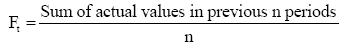
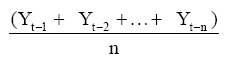
Forecasting method using single moving average: The single moving average method of forecasting is suitable for relatively stable time series with no trend or seasonal pattern. It involves calculating the average of observations and then employing that average as the predictor for the next period. The single moving average method is highly dependent on n which is the number of terms selected for constructing the average.
Single n period Moving Average
 .................... (Equation 1)
Where:
Ft is the forecast value for the next period,
Yt is the actual value at period t, and
n is the number of term in the single moving average based on the discretion of the researcher.
For single moving average, the 2, 4 and 6 yearly moving average was calculated and the forecast for the demand in year 2018 was obtained.
Forecasting method using simple exponential smoothing: The simple exponential smoothing method is a widely used and successful model which requires very little data. It is technique that uses weighted single moving average of past data as the basis for a forecast. This method keeps a running average of demand and adjusts it for each period in proportion to the difference between the latest actual demand figure and the latest value of the average. The derivation of equation for the simple exponential smoothing method is:
Ft = α Yt-1 + α (1 – α) Yt-2 + α (1 – α)2 Yt-3 +... ............. (Equation 2a)
Ft = α Yt-1 + α (1 – α) [α Yt-2 + α (1 – α) Yt-3 + ...]........ (Equation 2b)
Ft = α Yt-1 + (1 – α) Ft-1 ................... (Equation 2c)
Where:
Ft-1 is the last period forecast,
Ft is the forecast for period t.
Yt-1 is the last period actual value,
α is the smoothing constant (0 < α < 1),
The accuracy of simple exponential smoothing is dependent on the optimal value of α which is the smoothing constant. For the exponential smoothing, smoothing constants of 0.7, 0.8 and 0.9 was chosen and the forecast for the demand in year 2018 was calculated.
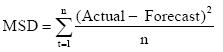
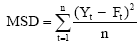
Mean squared deviation: When comparing the various forecasts, the Mean Squared Deviation (MSD) of the two forecasts was calculated and compared, and then the MSD that has a lower value was selected as preferred. The equation is:
 ..................................... (Equation 3)
Where:
Yt is the actual value in time period t
Ft is the forecast value in time period t
n is the number of periods
The results of this study will be in-line with the established objectives. The Table 1 below shows the demand for Nigeria international air passengers in the past seventeen years.
| Years | International Air Passenger Demand |
|---|---|
| Yr 2001 | 1,506,878 |
| Yr 2002 | 1,798,063 |
| Yr 2003 | 1,719,533 |
| Yr 2004 | 1,843,154 |
| Yr 2005 | 1,700,252 |
| Yr 2006 | 1,514,656 |
| Yr 2007 | 2,323949 |
| Yr 2008 | 2,557,264 |
| Yr 2009 | 2,619,918 |
| Yr 2010 | 3,217,876 |
| Yr 2011 | 3,586,742 |
| Yr 2012 | 4,440,930 |
| Yr 2013 | 4,600,698 |
| Yr 2014 | 4,654,941 |
| Yr 2015 | 4,233,844 |
| Yr 2016 | 4,260,989 |
| Yr 2017 | 3,575,542 |
Sources: Nigerian Civil Aviation Authority (2011); Federal Airport Authority of Nigeria (2017); Nigeria Bureau of Statistics (2018); Adeniran & Gbadamosi (2017).
Table 1: Demand for Nigeria international air passengers in the past seventeen years.
Forecasting for international air passenger demand in the year 2018 using single moving average
Equation 1 in the model specification has to do with forecasting method using single moving average. In order to derive the forecasts, the variables in the equation will be substituted with values.
Two (2) yearly moving average: The result of two yearly moving average was shown in Table 2 below.
| Years | International Air Passenger Demand | Two Yearly Moving Average |
|---|---|---|
| Yr 2001 | 1,506,878 | |
| Yr 2002 | 1,798,063 | |
| Yr 2003 | 1,719,533 | 1,652,471 |
| Yr 2004 | 1,843,154 | 1,758,798 |
| Yr 2005 | 1,700,252 | 1,781,344 |
| Yr 2006 | 1,514,656 | 1,771,703 |
| Yr 2007 | 2,323949 | 1,607,454 |
| Yr 2008 | 2,557,264 | 1,919,303 |
| Yr 2009 | 2,619,918 | 2,440,607 |
| Yr 2010 | 3,217,876 | 2,588,591 |
| Yr 2011 | 3,586,742 | 2,918,897 |
| Yr 2012 | 4,440,930 | 3,402,309 |
| Yr 2013 | 4,600,698 | 4,013,836 |
| Yr 2014 | 4,654,941 | 4,520,814 |
| Yr 2015 | 4,233,844 | 4,627,820 |
| Yr 2016 | 4,260,989 | 4,444,393 |
| Yr 2017 | 3,575,542 | 4,247,417 |
| Forecast 2018 | 3,918,266 |
Authors’ Computation (2018)
Table 2: Two yearly moving average forecast of international air passenger demand.
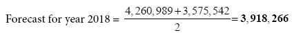
The forecast of demand in the year 2018 is the two yearly single moving average for the years before, hence 3,918,266. In the forecast, there were approximations because forecast cannot produce a fractional demand.
Four (4) yearly moving average: The result of four yearly moving average was shown in Table 3 below.
| Years | International Air Passenger Demand | Four Yearly Moving Average |
|---|---|---|
| Yr 2001 | 1,506,878 | |
| Yr 2002 | 1,798,063 | |
| Yr 2003 | 1,719,533 | |
| Yr 2004 | 1,843,154 | |
| Yr 2005 | 1,700,252 | 1,716,907 |
| Yr 2006 | 1,514,656 | 1,765,251 |
| Yr 2007 | 2,323949 | 1,694,399 |
| Yr 2008 | 2,557,264 | 1,845,503 |
| Yr 2009 | 2,619,918 | 2,024,030 |
| Yr 2010 | 3,217,876 | 2,253,947 |
| Yr 2011 | 3,586,742 | 2,679,752 |
| Yr 2012 | 4,440,930 | 2,995,450 |
| Yr 2013 | 4,600,698 | 3,466,367 |
| Yr 2014 | 4,654,941 | 3,961,562 |
| Yr 2015 | 4,233,844 | 4,320,828 |
| Yr 2016 | 4,260,989 | 4,482,603 |
| Yr 2017 | 3,575,542 | 4,437,618 |
| Forecast 2018 | 4,181,329 |
Authors’ Computation (2018)
Table 3: Four yearly moving average forecast of international air passenger demand.
Forecast for year 2018= 
The forecast of demand in the year 2018 is the four yearly single moving average for the years before, hence 4,181,329. In the forecast, there were approximations because forecast cannot produce a fractional demand.
Six (6) yearly moving average: The result of six yearly moving average was shown in Table 4 below.
| Years | International Air Passenger Demand | Six Yearly Moving Average |
|---|---|---|
| Yr 2001 | 1,506,878 | |
| Yr 2002 | 1,798,063 | |
| Yr 2003 | 1,719,533 | |
| Yr 2004 | 1,843,154 | |
| Yr 2005 | 1,700,252 | |
| Yr 2006 | 1,514,656 | |
| Yr 2007 | 2,323949 | 1,680,423 |
| Yr 2008 | 2,557,264 | 1,816,601 |
| Yr 2009 | 2,619,918 | 1,943,135 |
| Yr 2010 | 3,217,876 | 2,093,199 |
| Yr 2011 | 3,586,742 | 2,322,319 |
| Yr 2012 | 4,440,930 | 2,636,734 |
| Yr 2013 | 4,600,698 | 3,124,447 |
| Yr 2014 | 4,654,941 | 3,503,905 |
| Yr 2015 | 4,233,844 | 3,853,518 |
| Yr 2016 | 4,260,989 | 4,122,505 |
| Yr 2017 | 3,575,542 | 4,296,357 |
| Forecast 2018 | 4,294,491 |
Authors’ Computation (2018)
Table 4: Six yearly moving average forecast of international air passenger demand.
Forecast for year 2018 = 
The forecast of demand in the year 2018 is the six yearly single moving average for the years before, hence 4,294,491. In the forecast, there were approximations because forecast cannot produce a fractional demand.
Forecasting for International Air Passenger Demand in the Year 2018 Using Simple Exponential Smoothing
The model specification in equation 2c has to do with forecasting method using simple exponential smoothing. In order to derive the forecasts, the variables in the equation will be substituted with values.
Simple Exponential Smoothing with Smoothing Constant of 0.7: Forecast for year 2002 is the demand for year 2001 = 1,506,878 (Table 5).
| Years | International Air Passenger Demand | Exponential Smoothing 0.7 |
|---|---|---|
| Yr 2001 | 1,506,878 | |
| Yr 2002 | 1,798,063 | 1,506,878 |
| Yr 2003 | 1,719,533 | 1,710,708 |
| Yr 2004 | 1,843,154 | 1,716,885 |
| Yr 2005 | 1,700,252 | 1,805,273 |
| Yr 2006 | 1,514,656 | 1,731,758 |
| Yr 2007 | 2,323949 | 1,579,787 |
| Yr 2008 | 2,557,264 | 2,100,700 |
| Yr 2009 | 2,619,918 | 2,420,295 |
| Yr 2010 | 3,217,876 | 2,560,031 |
| Yr 2011 | 3,586,742 | 3,020,523 |
| Yr 2012 | 4,440,930 | 3,416,876 |
| Yr 2013 | 4,600,698 | 4,133,714 |
| Yr 2014 | 4,654,941 | 4,460,603 |
| Yr 2015 | 4,233,844 | 4,596,640 |
| Yr 2016 | 4,260,989 | 4,342,683 |
| Yr 2017 | 3,575,542 | 4,285,497 |
| Forecast 2018 | 3,788,529 |
Authors’ Computation (2018)
Table 5: Exponential smoothing (0.7) forecast of international air passenger demand.
Forecast for year 2018 = 0.7 (3,575,542) + 0.3 (4,285,497) = 3,788,529
The forecast of demand in the year 2018 is the average of the year 2017, hence 3,788,529. In the forecast, there were approximations because forecast cannot produce a fractional demand.
Simple Exponential Smoothing with Smoothing Constant of 0.8: Forecast for year 2002 is the demand for year 2001 = 1,506,878 (Table 6).
| Years | International Air Passenger Demand | Exponential Smoothing 0.8 |
|---|---|---|
| Yr 2001 | 1,506,878 | |
| Yr 2002 | 1,798,063 | 1,506,878 |
| Yr 2003 | 1,719,533 | 1,739,826 |
| Yr 2004 | 1,843,154 | 1,723,592 |
| Yr 2005 | 1,700,252 | 1,819,242 |
| Yr 2006 | 1,514,656 | 1,724,050 |
| Yr 2007 | 2,323949 | 1,556,535 |
| Yr 2008 | 2,557,264 | 2,170,466 |
| Yr 2009 | 2,619,918 | 2,479,904 |
| Yr 2010 | 3,217,876 | 2,591,915 |
| Yr 2011 | 3,586,742 | 3,092,684 |
| Yr 2012 | 4,440,930 | 3,487,930 |
| Yr 2013 | 4,600,698 | 4,250,330 |
| Yr 2014 | 4,654,941 | 4,530,624 |
| Yr 2015 | 4,233,844 | 4,630,078 |
| Yr 2016 | 4,260,989 | 4,313,091 |
| Yr 2017 | 3,575,542 | 4,271,409 |
| Forecast 2018 | 3,714,715 |
Authors’ Computation (2018)
Table 6: Exponential smoothing (0.8) forecast of international air passenger demand.
Forecast for year 2018 = 0.8 (3,575,542) + 0.2 (4,271,409) = 3,714,715
The forecast of demand in the year 2018 is the average of the year 2017, hence 3,714,715. In the forecast, there were approximations because forecast cannot produce a fractional demand.
Simple exponential smoothing with smoothing constant of 0.9: Forecast for year 2002 is the demand for year 2001 = 1,506,878 (Table 7).
| Years | International Air Passenger Demand | Exponential Smoothing 0.9 |
|---|---|---|
| Yr 2001 | 1,506,878 | |
| Yr 2002 | 1,798,063 | 1,506,878 |
| Yr 2003 | 1,719,533 | 1,768,945 |
| Yr 2004 | 1,843,154 | 1,724,474 |
| Yr 2005 | 1,700,252 | 1,831,286 |
| Yr 2006 | 1,514,656 | 1,713,355 |
| Yr 2007 | 2,323949 | 1,534,526 |
| Yr 2008 | 2,557,264 | 2,245,007 |
| Yr 2009 | 2,619,918 | 2,526,038 |
| Yr 2010 | 3,217,876 | 2,610,530 |
| Yr 2011 | 3,586,742 | 3,157,141 |
| Yr 2012 | 4,440,930 | 3,543,782 |
| Yr 2013 | 4,600,698 | 4,351,215 |
| Yr 2014 | 4,654,941 | 4,575,750 |
| Yr 2015 | 4,233,844 | 4,647,022 |
| Yr 2016 | 4,260,989 | 4,275,162 |
| Yr 2017 | 3,575,542 | 4,262,406 |
| Forecast 2018 | 3,644,228 |
Authors’ Computation (2018)
Table 7: Exponential smoothing (0.9) forecast of international air passenger demand.
Forecast for year 2002 is the demand for year 2001 = 1,506,878
Forecast for year 2018 = 0.9 (3,575,542) + 0.1 (4,262,406) = 3,644,228
The forecast of demand in the year 2018 is the average of the year 2017, hence 3,644,228. In the forecast, there were approximations because forecast cannot produce a fractional demand.
Determining the most appropriate forecasting method
This is done by comparing the yearly single moving averages with exponential smoothing of different smoothing constants. Before comparison using mean squared deviation, Figure 1 below is the line graph depicting the demand for international air passenger in Nigeria, the yearly single moving averages, and the simple exponential smoothing with different smoothing constants (Table 8).
| Years | International Air Passenger Demand | Two Yearly Moving Average | Four Yearly Moving Average | Six Yearly Moving Average | Exponential Smoothing 0.7 | Exponential Smoothing 0.8 | Exponential Smoothing 0.9 |
|---|---|---|---|---|---|---|---|
| Yr 2001 | 1,506,878 | ||||||
| Yr 2002 | 1,798,063 | 1,506,878 | 1,506,878 | 1,506,878 | |||
| Yr 2003 | 1,719,533 | 1,652,471 | 1,710,708 | 1,739,826 | 1,768,945 | ||
| Yr 2004 | 1,843,154 | 1,758,798 | 1,716,885 | 1,723,592 | 1,724,474 | ||
| Yr 2005 | 1,700,252 | 1,781,344 | 1,716,907 | 1,805,273 | 1,819,242 | 1,831,286 | |
| Yr 2006 | 1,514,656 | 1,771,703 | 1,765,251 | 1,731,758 | 1,724,050 | 1,713,355 | |
| Yr 2007 | 2,323949 | 1,607,454 | 1,694,399 | 1,680,423 | 1,579,787 | 1,556,535 | 1,534,526 |
| Yr 2008 | 2,557,264 | 1,919,303 | 1,845,503 | 1,816,601 | 2,100,700 | 2,170,466 | 2,245,007 |
| Yr 2009 | 2,619,918 | 2,440,607 | 2,024,030 | 1,943,135 | 2,420,295 | 2,479,904 | 2,526,038 |
| Yr 2010 | 3,217,876 | 2,588,591 | 2,253,947 | 2,093,199 | 2,560,031 | 2,591,915 | 2,610,530 |
| Yr 2011 | 3,586,742 | 2,918,897 | 2,679,752 | 2,322,319 | 3,020,523 | 3,092,684 | 3,157,141 |
| Yr 2012 | 4,440,930 | 3,402,309 | 2,995,450 | 2,636,734 | 3,416,876 | 3,487,930 | 3,543,782 |
| Yr 2013 | 4,600,698 | 4,013,836 | 3,466,367 | 3,124,447 | 4,133,714 | 4,250,330 | 4,351,215 |
| Yr 2014 | 4,654,941 | 4,520,814 | 3,961,562 | 3,503,905 | 4,460,603 | 4,530,624 | 4,575,750 |
| Yr 2015 | 4,233,844 | 4,627,820 | 4,320,828 | 3,853,518 | 4,596,640 | 4,630,078 | 4,647,022 |
| Yr 2016 | 4,260,989 | 4,444,393 | 4,482,603 | 4,122,505 | 4,342,683 | 4,313,091 | 4,275,162 |
| Yr 2017 | 3,575,542 | 4,247,417 | 4,437,618 | 4,296,357 | 4,285,497 | 4,271,409 | 4,262,406 |
| Forecast 2018 | 3,918,266 | 4,181,329 | 4,294,491 | 3,788,529 | 3,714,715 | 3,644,228 |
Source: Authors’ Computation (2018)
Table 8: Compressed results of Moving Average and Exponential Smoothing.
From Figure 2 above, it can be seen that most of the forecasts produced seems similar and difficult to identify the accurate forecast. Hence, to avoid this confusion, mean squared deviation was adopted for proper verification as to choose the most reliable forecasting method in this study.

Figure 2: Line graph depicting the comparison of international air passenger demand in Nigeria and results of different forecasts.
Equation 3 in the model specification has to do with mean squared deviation for comparison of the forecasting methods. In order to derive the forecasts, the variables in the equations will be substituted with values.
• The Table 9 below shows the MSD for two yearly single moving average.
| Years | International Air Passenger Demand (D) | Two Yearly Moving Average (E) | Deviation = D - E | Squared Deviation = (D – E)2 |
|---|---|---|---|---|
| Yr 2003 | 1,719,533 | 1,652,471 | 67,062 | 4497311844 |
| Yr 2004 | 1,843,154 | 1,758,798 | 84,356 | 7115934736 |
| Yr 2005 | 1,700,252 | 1,781,344 | -81,092 | 6575912464 |
| Yr 2006 | 1,514,656 | 1,771,703 | -257,047 | 66073160209 |
| Yr 2007 | 2,323949 | 1,607,454 | 716,495 | 5.13365E+11 |
| Yr 2008 | 2,557,264 | 1,919,303 | 637,961 | 4.06994E+11 |
| Yr 2009 | 2,619,918 | 2,440,607 | 179,311 | 32152434721 |
| Yr 2010 | 3,217,876 | 2,588,591 | 629,285 | 3.96E+11 |
| Yr 2011 | 3,586,742 | 2,918,897 | 667,845 | 4.46017E+11 |
| Yr 2012 | 4,440,930 | 3,402,309 | 1,038,621 | 1.07873E+12 |
| Yr 2013 | 4,600,698 | 4,013,836 | 586,862 | 3.44407E+11 |
| Yr 2014 | 4,654,941 | 4,520,814 | 134,127 | 17990052129 |
| Yr 2015 | 4,233,844 | 4,627,820 | -393,976 | 1.55217E+11 |
| Yr 2016 | 4,260,989 | 4,444,393 | -183,404 | 33637027216 |
| Yr 2017 | 3,575,542 | 4,247,417 | -671,875 | 4.51416E+11 |
| Summation | 3,960,191,404,001 |
Table 9: Mean Squared Deviation of two yearly moving average.
MSD for two yearly single moving average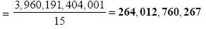
• The Table 10 below shows the MSD for four yearly single moving average.
| Years | International Air Passenger Demand (D) | Four Yearly Moving Average (E) | Deviation = D - E | Squared Deviation = (D – E)2 |
|---|---|---|---|---|
| Yr 2005 | 1,700,252 | 1,716,907 | -16,655 | 277389025 |
| Yr 2006 | 1,514,656 | 1,765,251 | -250,595 | 62797854025 |
| Yr 2007 | 2,323,949 | 1,694,399 | 629,550 | 3.96333E+11 |
| Yr 2008 | 2,557,264 | 1,845,503 | 711,761 | 5.06604E+11 |
| Yr 2009 | 2,619,918 | 2,024,030 | 595,888 | 3.55083E+11 |
| Yr 2010 | 3,217,876 | 2,253,947 | 963,929 | 9.29159E+11 |
| Yr 2011 | 3,586,742 | 2,679,752 | 906,990 | 8.22631E+11 |
| Yr 2012 | 4,440,930 | 2,995,450 | 1,445,480 | 2.08941E+12 |
| Yr 2013 | 4,600,698 | 3,466,367 | 1,134,331 | 1.28671E+12 |
| Yr 2014 | 4,654,941 | 3,961,562 | 693,379 | 4.80774E+11 |
| Yr 2015 | 4,233,844 | 4,320,828 | -86,984 | 7566216256 |
| Yr 2016 | 4,260,989 | 4,482,603 | -221,614 | 49112764996 |
| Yr 2017 | 3,575,542 | 4,437,618 | -862,076 | 7.43175E+11 |
| Summation | 7.72963E+12 |
Table 10: Mean Squared Deviation of four yearly moving average.
MSD for four yearly single moving average
• The Table 11 below shows the MSD for six yearly single moving average.
| Years | International Air Passenger Demand (D) | Six Yearly Moving Average (E) | Deviation = D - E | Squared Deviation = (D – E)2 |
|---|---|---|---|---|
| Yr 2007 | 2,323,949 | 1,680,423 | 643,526 | 4.14126E+11 |
| Yr 2008 | 2,557,264 | 1,816,601 | 740,663 | 5.48582E+11 |
| Yr 2009 | 2,619,918 | 1,943,135 | 676,783 | 4.58035E+11 |
| Yr 2010 | 3,217,876 | 2,093,199 | 1,124,677 | 1.2649E+12 |
| Yr 2011 | 3,586,742 | 2,322,319 | 1,264,423 | 1.59877E+12 |
| Yr 2012 | 4,440,930 | 2,636,734 | 1,804,196 | 3.25512E+12 |
| Yr 2013 | 4,600,698 | 3,124,447 | 1,476,251 | 2.17932E+12 |
| Yr 2014 | 4,654,941 | 3,503,905 | 1,151,036 | 1.32488E+12 |
| Yr 2015 | 4,233,844 | 3,853,518 | 380,326 | 1.44648E+11 |
| Yr 2016 | 4,260,989 | 4,122,505 | 138,484 | 19177818256 |
| Yr 2017 | 3,575,542 | 4,296,357 | -720,815 | 5.19574E+11 |
| Summation | 1.17271E+13 |
Table 11: Mean Squared Deviation of six yearly moving average.
MSD for six yearly single moving average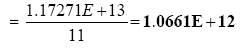
• The Table 12 below shows the MSD for simple exponential smoothing with smoothing constant of 0.7.
| Years | International Air Passenger Demand (D) | Exponential Smoothing of 0.7 (E) | Deviation = D - E | Squared Deviation = (D – E)2 |
|---|---|---|---|---|
| Yr 2002 | 1,798,063 | 1,506,878 | 291,185 | 84788704225 |
| Yr 2003 | 1,719,533 | 1,710,708 | 8,825 | 77880625 |
| Yr 2004 | 1,843,154 | 1,716,885 | 126,269 | 15943860361 |
| Yr 2005 | 1,700,252 | 1,805,273 | -105,021 | 11029410441 |
| Yr 2006 | 1,514,656 | 1,731,758 | -217,102 | 47133278404 |
| Yr 2007 | 2,323,949 | 1,579,787 | 744,162 | 5.53777E+11 |
| Yr 2008 | 2,557,264 | 2,100,700 | 456,564 | 2.08451E+11 |
| Yr 2009 | 2,619,918 | 2,420,295 | 199,623 | 39849342129 |
| Yr 2010 | 3,217,876 | 2,560,031 | 657,845 | 4.3276E+11 |
| Yr 2011 | 3,586,742 | 3,020,523 | 566,219 | 3.20604E+11 |
| Yr 2012 | 4,440,930 | 3,416,876 | 1,024,054 | 1.04869E+12 |
| Yr 2013 | 4,600,698 | 4,133,714 | 466,984 | 2.18074E+11 |
| Yr 2014 | 4,654,941 | 4,460,603 | 194,338 | 37767258244 |
| Yr 2015 | 4,233,844 | 4,596,640 | -362,796 | 1.31621E+11 |
| Yr 2016 | 4,260,989 | 4,342,683 | -81,694 | 6673909636 |
| Yr 2017 | 3,575,542 | 4,285,497 | -709,955 | 5.04036E+11 |
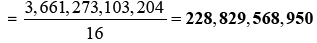
| Summation | 3,661,273,103,204 |
Source: Authors’ computation (2018)
Table 12: Mean Squared Deviation of exponential smoothing of 0.7.
MSD for simple exponential smoothing with smoothing constant of 0.7
• The Table 13 below shows the MSD for simple exponential smoothing with smoothing constant of 0.8.
| Years | International Air Passenger Demand (D) | Exponential Smoothing of 0.8 (E) | Deviation = D - E | Squared Deviation = (D – E)2 |
|---|---|---|---|---|
| Yr 2002 | 1,798,063 | 1,506,878 | 291,185 | 84788704225 |
| Yr 2003 | 1,719,533 | 1,739,826 | -20,293 | 411805849 |
| Yr 2004 | 1,843,154 | 1,723,592 | 119,562 | 14295071844 |
| Yr 2005 | 1,700,252 | 1,819,242 | -118,990 | 14158620100 |
| Yr 2006 | 1,514,656 | 1,724,050 | -209,394 | 43845847236 |
| Yr 2007 | 2,323,949 | 1,556,535 | 767,414 | 5.88924E+11 |
| Yr 2008 | 2,557,264 | 2,170,466 | 386,798 | 1.49613E+11 |
| Yr 2009 | 2,619,918 | 2,479,904 | 140,014 | 19603920196 |
| Yr 2010 | 3,217,876 | 2,591,915 | 625,961 | 3.91827E+11 |
| Yr 2011 | 3,586,742 | 3,092,684 | 494,058 | 2.44093E+11 |
| Yr 2012 | 4,440,930 | 3,487,930 | 953,000 | 9.08209E+11 |
| Yr 2013 | 4,600,698 | 4,250,330 | 350,368 | 1.22758E+11 |
| Yr 2014 | 4,654,941 | 4,530,624 | 124,317 | 15454716489 |
| Yr 2015 | 4,233,844 | 4,630,078 | -396,234 | 1.57001E+11 |
| Yr 2016 | 4,260,989 | 4,313,091 | -52,102 | 2714618404 |
| Yr 2017 | 3,575,542 | 4,271,409 | -695,867 | 4.84231E+11 |
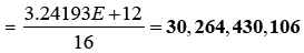
| Summation | 3.24193E+12 |
Source: Authors’ computation (2018)
Table 13: Mean Squared Deviation of exponential smoothing of 0.8.
• MSD for simple exponential smoothing with smoothing constant of 0.8
• The Table 14 below shows the MSD for simple exponential smoothing with smoothing constant of 0.9.
| Years | International Air Passenger Demand (D) | Exponential Smoothing of 0.9 (E) | Deviation = D - E | Squared Deviation = (D – E)2 |
|---|---|---|---|---|
| Yr 2002 | 1,798,063 | 1,506,878 | 291,185 | 84788704225 |
| Yr 2003 | 1,719,533 | 1,768,945 | -49,412 | 2441545744 |
| Yr 2004 | 1,843,154 | 1,724,474 | 118,680 | 14084942400 |
| Yr 2005 | 1,700,252 | 1,831,286 | -131,034 | 17169909156 |
| Yr 2006 | 1,514,656 | 1,713,355 | -198,699 | 39481292601 |
| Yr 2007 | 2,323,949 | 1,534,526 | 789,423 | 6.23189E+11 |
| Yr 2008 | 2,557,264 | 2,245,007 | 312,257 | 97504434049 |
| Yr 2009 | 2,619,918 | 2,526,038 | 93,880 | 8813454400 |
| Yr 2010 | 3,217,876 | 2,610,530 | 607,346 | 3.68869E+11 |
| Yr 2011 | 3,586,742 | 3,157,141 | 429,601 | 1.84557E+11 |
| Yr 2012 | 4,440,930 | 3,543,782 | 897,148 | 8.04875E+11 |
| Yr 2013 | 4,600,698 | 4,351,215 | 249,483 | 62241767289 |
| Yr 2014 | 4,654,941 | 4,575,750 | 79,191 | 6271214481 |
| Yr 2015 | 4,233,844 | 4,647,022 | -413,178 | 1.70716E+11 |
| Yr 2016 | 4,260,989 | 4,275,162 | -14,173 | 200873929 |
| Yr 2017 | 3,575,542 | 4,262,406 | -686,864 | 4.71782E+11 |
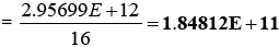
| Summation | 2.95699E+12 |
Source: Authors’ computation (2018)
Table 14: Mean Squared Deviation of exponential smoothing of 0.9.
• The Table 15 below shows the MSD for simple exponential smoothing with smoothing constant of 0.9.
| MSD of two yearly moving average | MSD of four yearly moving average | MSD of six yearly moving average | MSD of exponential smoothing constant 0.7 | MSD of exponential smoothing constant 0.8 | MSD of exponential smoothing constant 0.9 |
|---|---|---|---|---|---|
| 264,012,760,267 | 5.94587E+11 | 1.0661E+12 | 228,829,568,950 | 30,264,430,106 | 1.84812E+11 |
Source: Authors’ computation (2018)
Table 15: Comparison of MSDs for two, four, and six yearly single moving averages, simple exponential smoothing constants of 0.7, 0.8, and 0.9.
From the comparison of the different MSDs shown in Table 15 and Figure 3 respectively, it can be seen that the MSD of exponential smoothing with constant 0.8 appears to give the best year 2018 forecasts as it has a lower MSD than all other forecasting methods. Hence, the 2018 forecast of 3,714,715 that was produced by exponential smoothing with constant 0.8 was preferred (Figure 3).

Figure 3: Pictorial view comparing MSDs of forecasting methods.
In conclusion, this study examined the dynamics for evaluating different forecasting methods for international air passenger demand in Nigeria. Yearly data from 2001 to 2017 were collected and used to forecast the year 2018 international air passenger demand in Nigeria.
Lastly, the study revealed that simple exponential smoothing with constant 0.8 is closer to the original raw data; hence, it can be said that exponential smoothing with constant 0.8 will give a better forecast for the demand in year 2018 and subsequent years if adopted. The evaluation statement was best justified in the third objective where the mean square deviation was adopted to compare the different methods of forecast, so the year 2018 forecast of 3,714,715 was preferred.