Journal of Research and Development
Open Access

The Effect of Job Destruction Shocks in Unemployment Theory

Walid Y Alali^* and John Knight ^*Correspondence: Walid Y Alali, Department of Economic, University of Oxford, Manor Road Building, OXI 3UQ, Oxford, United Kingdom, Email:

Author info »

Introduction

This paper explores how the dynamics of unemployment, as described by the Diamond Mortensen-Pissarides framework, undergo a fundamental change when we loosen the assumption of free entry of vacancies. This is significant because we demonstrate that a key implication of the free entry approach, which states that tightness of the market is unrelated to unemployment when productivity variables are taken into account, does not align with the data. Additionally, by considering a vacancy creation process that is not infinitely elastic, we illustrate why vacancies decrease as unemployment rises following a recession-induced job separation shock. This dynamic response is important because it eliminates the need to impose an arbitrary restriction of zero job separation shocks in order to generate correlations in the Beveridge curve. Moreover, once we allow for an exogenous job separation process that is relevant to the data, the relaxed framework reveals that the assumption of the small surplus is no longer necessary to explain the level of volatility in unemployment. This finding challenges the findings of previous studies such as [1,2]. Through various tests, we demonstrate the improved empirical properties of this relaxed approach compared to the free-entry approach.

According to the structural model, the main factor behind the fluctuation in unemployment throughout the economic cycle is the process of job separation.

The groundbreaking contribution made by Mortensen and Pissarides, henceforth referred to as MP, was their discovery of an equilibrium model of unemployment that aligns with three key characteristics of the business cycle [3]. These characteristics are as follows: (MP1) There is a negative correlation between the flows of job destruction and job creation, (MP2) job destruction flows have a higher level of variability compared to job creation flows, and (MP3) job destruction exhibits an asymmetrical pattern, with a rapid increase at the onset of a recession. This is also discussed in the work of Davis and Haltiwanger, the recent survey conducted by Elsby et al, and Figures 4 and 5 provided below, which pertain to the Great Recession [4,5]. In our study, we focus on job separation shocks instead of on-the-job searches. These shocks describe the movement of employed individuals into unemployment. It is important to note that while job destruction shocks are related, they are not the same. In the presence of an on-the-job search, a job is considered destroyed when an employee resigns to pursue alternative employment and the firm does not hire a replacement. Shimer has raised three challenges to the MP framework [6]. Firstly, it generates insufficient persistence in unemployment. Secondly, when the productivity process is properly calibrated, it results in inadequate volatility of unemployment. Lastly, the shocks of the large job separation lead to a counterfactual positive correlation between unemployment and vacancies.

Shimer, Hall, and Hagedorn and Manovskii all discuss the equilibrium unemployment literature [1,6,7,]. One common assumption in this literature is that there are no shocks to aggregate job separation and that there is a small surplus. While this assumption addresses some of the criticisms raised by Shimer, it is not consistent with the idea that job creation flows have a higher variance than job separation flows. Our paper aims to find an approach that is fully consistent with all these considerations.

The assumption that vacancies have free entry is quite strong because it suggests that even a small increase in productivity will immediately lead to a surge in the number of open positions. However, this assumption does not align with the data, as demonstrated by Sniekers [8]. In order to address this, we adopt a job creation process similar to Diamond and Fujita and Ramey [9,10]. In this process, creating a new job requires an initial investment in new technology, and the cost of this investment is randomly drawn from an external distribution. This approach, which we refer to as the “Diamond entry” process, includes the assumption of free entry as a special case. However, considering a finite number of firms with varying investment costs also allows for a vacancy creation process that is not infinitely elastic. The level of elasticity is crucial in explaining the dynamics of equilibrium unemployment, which is why we use the SMM (Simulated Method of Moments) to identify it. We base our analysis on target moments from Shimer that describe the cyclical patterns of unemployment, vacancies, and market tightness [6]. Through SMM, we find that the process of vacancy creation is not infinitely elastic, which has significant implications.

There has been a significant rise in job openings. In fact, the way job vacancies are created, without flexibility, leads to the continued presence of unemployment, which is not seen in the approach where entry into the job market is unrestricted. When unemployment increases, the creation of job openings is less pronounced, resulting in lower rates of finding employment and therefore more enduring unemployment. This also fundamentally alters how the economy responds to a sudden loss of jobs.

When there are major job separations that allow anyone to enter the job market freely, it creates a situation where unemployment and job vacancies are positively correlated. However, this is not the case when there are specific entry conditions in place. In our calibrated model, we find that after a single job separation shock, the stock of vacancies decreases because the influx of laid-off workers depletes the existing vacancies. As a result, unemployment increases, and the declining vacancy stock leads to a decrease in worker job finding rates. These unemployment dynamics align with the insights of Shimer (2005) and (2012), as well as with the U.S. unemployment dynamics following the great recession [6,11].

The structure of this paper is as follows: Section 2 describes the model, while Section 3 characterizes its (Markov) equilibrium. Section 4 includes the calibration exercise and examines various tests that compare the properties of our model to the free entry/small surplus/ no job separation shocks approach. Additionally, Elsby et al., present a different test that supports our approach [5]. Section 6 employs the calibrated model to examine how the Great Recession affected the outcomes in the US labour market. However, instead of using a different metric to measure job separation shocks, it utilizes layoffs taken from JOLTS. The conclusion is covered in section 7, while section 8 includes the data appendix.

Methodology

The model

In our analysis, we adopt a traditional model of unemployment that considers discrete time and an infinite time horizon, as exemplified by [12]. All firms and workers are assumed to have equal productivity, and they all offer the same wage based on Nash bargaining. Each workerfirm pairing continues until a job separation shock disrupts it. In this scenario, vacancies are regarded as a fixed quantity and are not easily replenished. Without the freedom for new participants to enter, the levels of vacancies and unemployment become significant factors in the overall state of affairs.

We introduce a finite and fixed measure F>0 to represent the number of firms that generate vacancies. In each period, every firm encounters one new and independent business opportunity.

When given the chance, the company assesses the cost of its investment, x, in relation to the expected return. The expected return is influenced by the overall state of the economy at a given time t, which is represented as Ω_t and will be described in detail later. We use to represent the anticipated return of a business opportunity in the state Ω_t. The investment cost, x, is a random draw from a cost distribution called H, which is independent of the company. For simplicity, we assume that this investment cost encompasses all the unique aspects associated with a particular business venture. In other words, more profitable opportunities are linked to lower values of x. If the company decides to invest, it incurs the sunk cost x and gains an unfilled job with an expected value of J_t. Essentially, each new investment creates one new job vacancy.

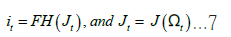
In accordance with Diamond’s research, every company invests in a business opportunity only if it holds positive value, meaning that x ≤ J_t . This eliminates the need to remember a business opportunity if the company decides not to invest immediately. As investments are made whenever x ≤ J_t , the aggregate level of new vacancy creation in period t can be described as . To explain how a company fills a vacancy, we will use the standard matching framework (without free entry). There is a fixed number of workers who are assumed to have infinite lifespans. Both workers and companies have the same level of risk aversion and discount factor, with a value between 0 < β < 1. Workers switch between being employed and unemployed based on their labour market outcomes. The cost of posting an unfilled vacancy is represented by c ≥ 0 . Each period is defined by the number of vacancies (unfilled jobs) represented by v_t , and the number of unemployed workers represented by u_t (with 1−u_t indicating the number of employed workers). The hiring process is characterized by friction, meaning that the number of new job-worker matches in period t, represented by m_t, is determined by a matching function . This function m(.) is positive, increasing, concave, and homogeneous of degree one. In each period, there is a positive payoff z>0 for jobworker matches. The market output t p = p remains the same for each match in period t, while the overall productivity t p changes based on an external AR1 process. The process of job separations, whether the job is filled or unfilled, is also external and random. The probability of a job being destroyed is denoted as t δ . If a filled job is destroyed, the worker becomes unemployed and the job’s continuation payoff is zero. Now, let’s move on to the events that occur within each period t. Each of these Period have five stages as follows:

New realisations: In the previous period, we were given Now, we have new values for p_t and δ_t . To determine pt, we use the equation The values of are random noises drawn from a normal distribution with a mean of zero and a covariance matrix Σ , δ ≤ 0. The long-run average job separation rate, δ , is greater than zero, and the long-run productivity, p, is normalized to one.

Bargaining and production: The wage, w_t , is determined through Nash bargaining. During this stage, production takes place, and when a job match occurs, the profit for that period is for the employer, and the employed worker receives a payoff of t w . Each unemployed worker receives a payoff of z.

Vacancy investment: Firms invest in creating new vacancies, which we denote as i_t .

Matching: At the beginning of this stage, there are stocks of unemployed job seekers and vacancies, u_t , and v_t respectively. The matching process occurs, resulting in which represents the total number of new matches.

Job separation: During this stage, each vacancy and filled job has an independent probability of being destroyed, which is denoted as δ_t.

The equilibrium of dynamics markov mode

This section presents the equilibrium dynamics of the Markov model. In this model, the variable u_t represents the number of unemployed individuals in period t just before the matching stage (stage IV). The evolution of u_t can be described by the following equation:

Here in, , the second term represents the number of employed workers in period t-1 who become unemployed due to a job separation shock. The last term represents the outflow of matches, which is also affected by the job separation shock in period t-1. The dynamics of the vacancy stock can be described as follows:

The first term in this equation represents the vacancies that were not filled in the previous matching event, while the second term represents the creation of new vacancies (i_t).

In order to determine the equilibrium creation of new vacancies, we focus on Markov equilibria. Once the values of are determined, we can define the intermediate stock of vacancies as This represents the number of vacancies that survive from the previous matching event. When bargaining takes place in stage II, we can denote the corresponding state space as . Nash bargaining procedure yields a wage rule of the form . 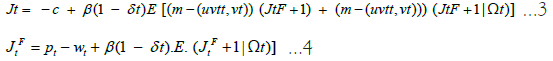Stage III determines optimal investment ,matching and separation dynamics ensure Ω_t evolves as a first-order Markov process, Ω_t is indeed a sufficient statistic for optimal decision making in period t. Additionally, we will analyze the Bellman equations that govern optimal behaviour in period t, specifically at the beginning of stage II when the state vector is Ω_t . represents the anticipated worth of the value of vacancy. While represents the anticipated worth of field job value. 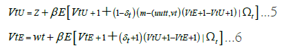represents the worker’s expected value of being unemployed, and represents the worker’s expected worth of employed value. Let represents the expectations operator given the state vector (Ω_t) at period t. The model’s timing suggests that the value functions are defined recursively.

In mean time the function of worker value defined respectively

businesses only invest when the cost of the opportunity is x ≤ J_t . In equilibrium, the creation of new job vacancies, it, depends on the function i_t = i .Ω_t then

the assumption that workers possess a certain level of bargaining power, denoted by the variable Ï? , which falls within the range of values between 0 and 1. The axiomatic Nash bargaining approach then concludes the model by incorporating this assumption. By using

equation which is determined equilibrium wages. Therefore, we have a set of self-governing equations of the first degree that establish (i) the progression of (Ω_t) and (ii) the equilibrium value functions with their respective investment guideline

Calibration and trial

To calibrate the model using the data discussed in Shimer’s work, we follow the standard framework and utilize the calibration parameters outlined in Mortensen and Nagypal’s study [6,13]. In this calibration, we assume that each period represents a month and employ a conventional Cobb-Douglas matching function, denoted as The parameter values for Mortensen and Nagypal’s framework are summarized in (Table 1).

Table 1: Mortensen/nagypal parameters.

The Hosios condition is met, indicating that the mean value of the productivity process for p_t is equal to one in the long run. This means that the surplus, which is equal to (1-z)/z=43%, is significant. Based on the monthly discount factor, the annual discount rate is determined to be 4%. Instead of assuming the job separation shocks equal zero, we calibrate the process to align with the data described in Shimer [6]. Figure 1 illustrates the extent of log-deviations in job separation rates and labor productivity, as computed for the Shimer data at frequencies corresponding to business cycles [6]. The data appendix provides an explanation of how Shimer measures the job separation rate [6]. Since the data is recorded only on a quarterly basis while the model operates on a monthly time structure, we select the autocorrelation parameters , and covariance matrix Σ in such a way that the resulting process , when reported quarterly, matches the first-order autocorrelation and cross correlation indicated by the data. By doing this, we are able to achieve (Figure 1).

Figure 1: U.S. separation rates and labor productivity (1951-2003)4. Note:

By conducting analyses at regular intervals, we can observe the expected first-order autocorrelation and cross-correlation as suggested by the data. This process results in the following findings (Table 2).

Table 2: Monthly frequencies stochastic process.

As shown in Figure 1, and in line with the viewpoint expressed in MP, there is a clear inverse relationship between job separation innovations and productivity innovations. Additionally, the variance of job separation innovations is significantly higher. It is important to note that MP discusses both the endogenous job destruction margin and a single exogenous stochastic process for (p_t) . When calibrating a DMP framework, it is commonly observed that the cost of posting vacancies, denoted as c, needs to be relatively high. This is often justified by the argument that it represents prior investments made in job creation. However, in this case, we present the opposite scenario.

Instead of considering small costs for posting vacancies, we assume that there are no costs at all (c=0). This means that all the costs associated with creating jobs are related to the investment decision made beforehand. According to the rule for creating vacancies, , we simplify the functional form by using the most basic and straightforward equation:

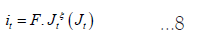
In this equation, ξ represents the elasticity of new vacancy creation in relation to the value of the vacancy. If ξ = ∞ , it means that new vacancy creation is infinitely elastic, similar to a situation of free entry. On the other hand, if ξ = 0, it implies that new vacancy creation is perfectly inelastic or fixed. We calibrate the framework to match the average turnover rates in the long run. To ensure that our results can be compared with others, we follow Shimer’s suggestion that the probability of job separation should be 3.4% per month, and the average duration of an unemployment spell is 2.2 months, resulting in a long-run unemployment rate of u=7%. It is also worth mentioning that the average duration of vacancies is approximately 3 weeks, as noted by Blanchard and Diamond (1989) [6,14]. By imposing these restrictions, we determine that δ . The mean monthly job separation rate, is equal to the (δ = 0.034) . Which represents the average monthly job separation. The subsequent restrictions, depending on the chosen value of ξ , determine the scale parameter values of A (matching function) and F (vacancy creation rule). To illustrate, if ξ is set to 1, indicating a uniform distribution of investment costs, A is determined to be 0.594 and F is determined to be 0.0075. This leaves us with one remaining parameter, ξ , which represents the elasticity of the job creation process. We estimate the value of ξ using the SMM, as outlined in Ruge-Murcia’s methodology, employing a Newey-West diagonal weighting matrix [15]. For each chosen value of ξ , we adjust the values of parameters (A, F) to ensure that the generated data aligns with the long-term turnover means. The target moments used to identify ξ are derived from the standard deviations and correlations of unemployment, vacancies, and market tightness, as presented in Table 1 of Shimer [6].

Results and Discussion

The data targets are recorded in Column 1 of Table 3, where the Beveridge Curve (BC) shows the inverse relationship between vacancies and unemployment. The remaining columns provide statistics based on model-generated data. Let’s focus on the final column, which is labelled H/M. In this column, we assume free entry and set certain values such as Ζ=0.955 (representing a small surplus), φ = 0.052 (indicating low worker bargaining power), and δ_t =δ (no separation shocks), as discussed in Hagedorn’s and Manovskii, to ensure comparability of results, we will keep the Mortensen/Nagypal parameter values the same, with x set to 0 [13]. We will calibrate c to match the long-run turnover means, resulting in c=0.63. However, Hagedorn and Manovskii have chosen different values for γ ,δ , and c, with γ = 0.41, δ = 0.026 , and c=0.58 (Table 3) [1].

Table 3: Simulation results.

This specification produces the Beveridge curve [BC] and achieves favourable volatility outcomes. The column labelled “H/M with JD” enhances the H/M specification by incorporating the process of job separation (with appropriate recalibration). Including separation shocks leads to greater volatility in unemployment, but, as argued by Shimer, it reduces the strong negative correlation between unemployment and vacancies also highlight this point and explore the role of on-the-job search in mitigating this issue) [6,16]. The column ξ =1presents the results when the process of vacancy creation is assumed to be unit elastic. Under this assumption, the model produces the correct correlated behaviour, but there is insufficient volatility. To match the desired volatility targets, SMM suggests that the process of vacancy creation must be less than unit elastic, with an estimated value of ξ = 0.265. Although ξ = 0.265slightly exaggerates the negative correlation between unemployment and vacancies, it perfectly fits the chosen targets in terms of volatility.

Next, we examine three tests that highlight the distinct dynamic properties of our relaxed approach compared to the free entry case. In Section 6, we utilize these insights to analyse the unemployment dynamics following the Great Recession. Referring to the data in Table 1, Shimer, and the accompanying table for the case ξ = 0.265, it is crucial to mention that market tightness and unemployment have a remarkably strong negative correlation of 0.97 (also shown in Table 3) [6]. On the other hand, the correlation between market tightness and productivity is only 0.40, while the correlation with job separation rates is -0.71.

Test 1- market tightness dynamics

The relationship between worker job-finding rates and market tightness determines how the market fluctuates. By using a free entry approach, we can simplify the equilibrium market tightness . and make it independent of unemployment U_t. However, when considering we can conduct a statistical test to determine if market tightness θ_t is truly unrelated to unemployment. Our goal is to see if the market tightness dynamics generated by the model align with the actual data. In Table 4, Column 1 (Data), we present the results of estimating a log-linear statistical relationship.

Table 4: Reduced form market tightness dynamics.

Using Shimer HP filtered data [6]. To address simultaneity concerns due to market tightness being measured as we use last period as the conditioning variable. (Using log U_t as the conditioning variable reveals that estimated productivity effects (δ_t) become negative and insignificant, and there is an even stronger negative correlation between unemployment and measured market tightness). The estimated t-statistics are enclosed in brackets (Table 4). Based on the data (column 1), we observe a positive correlation between market tightness and productivity, as well as a negative correlation between market tightness and job separation rates. However, the significance of productivity shocks is minimal (t-statistic equal to 1). The correlation between unemployment and market tightness is robust, as indicated by a t-statistic of -26. In Section 6, Figure 5 visually supports this finding by illustrating the evolution of market tightness after the 2008 Great Recession. The final column, labelled as H/M with JD, presents the results obtained from the free entry/small surplus approach, combined with the process of job separation described above. In this approach, market tightness is primarily influenced by productivity shocks, with small surplus and free entry contributing to the opposite scenario. Additionally, given market tightness not dependent on unemployment. While not identical, a parameter estimates of ξ = 0.265 aligns reasonably well with the data, indicating a strong correlation between market tightness and unemployment, along with significant contributions from productivity and job separation shocks.

Test 2, titled-serial persistence

Raises an important critique made by Shimer regarding the lack of sufficient persistence in the MP framework [6]. In Table 5, the first column, labelled “Data,” displays the serial autocorrelation of unemployment, vacancies, and market tightness based on the filtered data using the HP method. The remaining columns provide the parameter estimates for these variables using model-generated data. Upon analysing the data at quarterly frequencies, we find that the implied serial persistence parameters for productivity and job separation rates are respectively. Comparing this to the first column of Table 5, it becomes evident that unemployment, vacancies, and market tightness exhibit much stronger persistence (Table 5).

Table 5: Estimated serial persistence (Quarterly frequencies).

When considering the H/M with the JD model, it is observed that there is no additional persistence in unemployment beyond that of the underlying productivity process. This can be attributed to the fact that a free entry specification implies and without any feedback from unemployment to market tightness, the small surplus assumption leads to unemployment having a persistence of which is deemed too low. However, with a value of ξ = 0.265, the second column of Table 5 demonstrates that the serial persistence of closely matches the data. This is because, as showcased in Table 4, market tightness exhibits a strong negative correlation with unemployment.

Our third test focuses on the persistence of high unemployment caused by below-average job finding rates. The level of persistence, known as , is determined by the model’s propagation mechanism. In the next section, we will delve into the details of this mechanism.

Test 3-the unemployment (Ins and outs)

According to Shimer, the connection between unemployment and job rates is stronger than the connection between unemployment and job separations [11]. The argument starts by acknowledging that steady state unemployment is determined by the rate at which employed workers transition into unemployment and the rate at which unemployed workers find employment . It is then suggested that the proxy variable for unemployment

which is calculated using the exit rate (x_t) and job finding rate (f_t) at a given period (t), is a reasonable approximation for actual unemployment (u_t). This proxy variable (u_t^P ) can be further broken down into the effects of job separations (variations in x_t) and job finding (variations in f_t). For instance, when the sequence represents the variation in u_t^P solely due to changes in describes the variation in u_t^P caused by changes in x_t. Shimer defines the contribution of the job-finding rate to unemployment variations as the covariance of u_t and divided by the variance of u_t [11]. According to Elsby, Fujita and Ramey, only 24% of the contribution is made [17,18]. This aligns with the small surplus/free entry approach, as significant fluctuations in job creation result in corresponding fluctuations in unemployment and worker job-finding rates. To validate this, we apply the Shimer methodology to model generated data using = 0.265, [11]. By computing the same statistics, we find that job-finding variations account for 77% of the unemployment variation, while job separation variations, contribute slightly less at 21%. Thus, the properties of the simulated data support the Shimer decomposition [11]. However, we demonstrate that job separation shocks drive the volatility of unemployment in the structural model.

How significant a role do job separation shocks play in the variation of unemployment?

The previous explanation has demonstrated that our framework not only aligns well with the fluctuations, connections, and persistence of market tightness, unemployment, and vacancies, but it also fully corresponds with the breakdown of unemployment by Shimer [11]. So, the interesting question becomes: how significant are job separation shocks in explaining the volatility of unemployment? To address this, we can assume job separation shocks is zero , adjust the productivity process accordingly, and reevaluate ξ . By doing so, we find that unemployment volatility , which is only a quarter of what is observed in the data (SMM maximizes unemployment volatility by setting ξ arbitrarily high in the absence of separation shocks, adhering to the free entry assumption). This outcome shouldn’t come as a surprise since Figure 1 illustrates that productivity shocks are minimal, and we haven’t specified a small surplus. However, it remains a question of how this DMP framework, where job separation shocks drive unemployment volatility, aligns with both the Beveridge curve and the Shimer breakdown (Figure 2) [11].

Let’s consider Figures 2 and 3. Figure 2 outlines the immediate response of unemployment to a single separation innovation at time zero (while keeping productivity constant at p_t = 1).

Figure 2: Impulse response of unemployment to a separation shock. Note: Unemployment, H/M with JD, Separation.

We also map the distribution process of the exogenous AR1 locus δt . The impulse response function, (H/M with JD), describes the impulse response of unemployment under conditions of free entry and marginal surplus. These shocks result in relatively small increases in unemployment, and unemployment rates appear to be as stable as the divorce rate. In contrast, ξ = 0.265gives a much larger unemployment peak and much greater stability. Figure 3, which illustrates the associated impulse response of the air gap, shows why (Figure 3).

Figure 3: Impulse response of vacancies to a separation shock. Note: Unemployment, H/M with JD, Separation.

Free entry (H/M with JD) with a small surplus means increasing vacancies due to rising unemployment. Addressing these gaps could quickly bring unemployment to long-term stability. This adjustment process also means that unemployment and job vacancies change positively, which is inconsistent with a Beveridge curve. Contrary to ξ = 0.265, Figure 3 shows that job vacancies decrease as the rate of unemployment increasing. The initial iteration in Figure 3 is influenced by the model’s expected time. For open access, a high labor allocation ratio δ t (which is known in stage I, but the allocation occurs only in stage V) reduces the market density in stage III. Since the rate of unemployment in Step 3 is the trend during the first iteration, the low market density means that vacancies are below the trend in the first iteration but increase as the unemployment rate increases. Conversely, at ξ = 0.265, job creation is always above trend (this causes the rate of unemployment to return to trend). In the first two iterations, the vacancy base (measured in three phases before job losses) is slightly above trend. However, rapid increases in unemployment and hiring reduce the stock of vacancies and begin to recover once the stock of vacancies falls below the unemployment peak.

Job fragmentation shocks not only eliminate some vacancies but also increase waves of the unemployed, some of whom quickly join the existing labor pool. In the rigid job creation process, oversampling the job pool of newly laid off workers will reduce the number of jobs. As more and more unemployed people look for jobs that are missing, the number of unemployed job seekers will gradually decrease.

Therefore, this dynamic yields results consistent with those in the Shimer [11]. Because division of labor shocks that drive recessions but are short-lived produce persistently high unemployment and persistently low unemployment. Without introducing any job allocation shock, the calibrated model can find that the job allocation process drives the volatility of unemployment.

The great recession 2008/9

The 2008/9 Great Recession serves as a perfect example to showcase the effectiveness of this approach when analysing the aggregate labour market dynamics in the United States. By examining the CPS data and referring to Figure 4, we can observe the seasonally adjusted gross hires, gross job separations, and non-farm layoffs from JOLTS, a time series that has been available since 2001. Figure 4 provides us with valuable insights into the significant increase in layoffs during the 2008-2009 Great Recession. Based on the free entry approach, one would expect vacancies to increase and hires to surge following such a shock. However, this was not the case. Instead, in line with our approach, the shock of job separations resulted in a steep decline in the stock of vacancies as unemployment rates rose. To delve deeper into the evolution of the U.S. labor market during and after the spike in layoffs in 2008/9, we turn to Figure 5. Using the Shimer methodology, this figure examines unemployment, market tightness, productivity, and layoffs [6]. Each of these factors is measured as log deviations from the trend, employing an HP filter with a smoothing parameter of 105. At the onset of the layoff spike, the market tightness slightly exceeded the trend, while unemployment rates were slightly below it.

Figure 4: U.S. Job turnover from 2000 to 2015. Note: Separation, Layoffs from JOLTS.

Figure 5: U.S. labor market indicators from 2008 to 2015. Note: Unemployment, Market tightness, Layoffs.

The graph shows a significant decline in market tightness. Surprisingly, productivity was actually correlated with unemployment during this period from 2008 to 2015 (Figure 4).

According to the theory of free entry and small surplus, market tightness should have been correlated with unemployment in a positive way. However, Figure 5 disproves this theory and demonstrates a strong negative correlation between market tightness and unemployment. Additionally, despite high unemployment and above-average productivity after 2010, the vacancy stock and gross hires did not exceed the expected trend as predicted by the theory of free entry (Figure 5).

Figure 4 confirms this by showing that hire flows only returned to the expected trend. Therefore, it is difficult to explain the post-2008 changes in the U.S. economy using the freeentry approach. On the other hand, the impulse response functions (Figures 2 and 3) show consistent behaviour following a job separation shock, unlike the ξ = 0.265scenario (Table 6).

Table 6: Simulation Results for JOLTS calibration.

To further analyse the data from 2001 to 2015, we use the JOLTS layoff series as a more direct measure of the process of job separation proposed [19-23]. Although the spike in layoffs in 2008/2009 does not align with a stationary AR1 process, we continue with the same methodology. To align the data, we adjusted ρ_p , ρ_δ , and the covariance matrix Σ . This involved setting ρ_p to 0.95, ρ_δ to 0.89 with σ_p to 0.0063, σ_δ to 0.036, and the cross correlation ρ_pδ to -0.38 monthly. The updated targets are shown in the first column of Table 6. Additionally, finding third column displays the statistics derived from model-generated data using the previously estimated ξ value of 0.265 [24-29].

Using model-generated data with a previously estimated value of ξ = 0.265, column 3 presents the corresponding statistics. It is not surprising that this specification, given its close resemblance to the data in Figures 2 and 3, continues to fit the joint correlations of unemployment, vacancies, and market tightness quite well. However, this time, the value of ξ = 0.265results in insufficient volatility in unemployment [30-36]. This is due to the fact that a less elastic process for creating vacancies leads to lower job-finding rates following a significant layoff shock. As a result, the method of estimation this time yields a value of ξ = 0, indicating perfectly inelastic vacancy creation rates [37-40]. This is partially supported by Figure 4, which shows that hires returned to the trend after the spike in layoffs, resulting in a so- called jobless recovery. Nonetheless, even with ξ = 0, this approach still fails to capture sufficient volatility in unemployment during this period [41,42].

Conclusion

This paper has highlighted the empirical challenges that arise from assuming the unrestricted entry of vacancies in the DMP framework. Specifically, the notion that market tightness is orthogonal to unemployment, given productivity variables, is not supported by the data.

The use of SMM estimation reveals that the process of creating job vacancies is not flexible. This new equilibrium framework aligns with the findings of Shimer and the perspectives of Mortensen and Pissarides on job creation and job separation patterns during economic cycles. The results indicate that the assumption of the job separation shocks equal zero is not valid, as it is actually the process of job separation that influences the volatility of unemployment over the cycle. This approach provides a straightforward explanation for the observed dynamics of unemployment and job vacancies in the U.S. post the Great Recession. Our approach opens up new avenues for future research. For instance, what are the economic factors that drive the process of job separation? Mortensen and Pissarides propose that adverse aggregate productivity shocks lead to bursts of job destruction. However, the Great Recession suggests that financial or credit shocks may also play a significant role, as suggested. In order to avoid closing down, companies must reduce their size. It is important to have more concrete evidence of the vacancy creation elasticity ξ , as it greatly influences the behavior of the economy. By eliminating the assumption of a small surplus, the equilibrium DMP framework becomes applicable for policy analysis once again, as shown.

References

1. Hagedorn M, Manovskii I. The cyclical behavior of equilibrium unemployment and vacancies revisited. Am Econ Rev. 2008;98(4):1692-1706.

   [Crossref] [Google Scholar]

2. Ljungqvist L, Sargent TJ. The fundamental surplus. Am Econ Rev. 2017;107(9):2630-2665.

   [Crossref] [Google Scholar]

3. Mortensen DT, Pissarides CA. Job creation and job destruction in the theory of unemployment. Rev Econ Stud. 1994;61(3):397-415.

   [Crossref] [Google Scholar]

4. Davis SJ, Haltiwanger J. Gross job creation, gross job destruction, and employment reallocation. Quart J Econ. 1992;107(3):819-863.

   [Crossref] [Google Scholar]

5. Elsby MW, Michaels R, Ratner D. The Beveridge curve: A survey. J Econ Literat. 2015;53(3):571-630.

   [Crossref] [Google Scholar]

6. Shimer R. The cyclical behavior of equilibrium unemployment and vacancies. Am Econ Rev. 2005;95(1):25-49.

   [Crossref] [Google Scholar]

7. Hall RE. Job loss, job finding, and unemployment in the US economy over the past fifty years. NBER Macroecon Ann. 2005;20:101-137.

   [Crossref] [Google Scholar]

8. Sniekers F. Persistence and volatility of beveridge cycles. Int Econ Rev. 2018;59(2):665-698.

   [Crossref] [Google Scholar]

9. Diamond PA. Aggregate demand management in search equilibrium. J Politl Econ. 1982;90(5):881-894.

   [Crossref] [Google Scholar]

10. Fujita S, Ramey G. The dynamic beveridge curve. 2005.

    [Crossref] [Google Scholar]

11. Shimer R. Reassessing the ins and outs of unemployment. Rev Econ Dynam. 2012;15(2):127-148.

    [Crossref] [Google Scholar]

12. Pissarides CA. Equilibrium unemployment theory. 2000.

    [Google Scholar]

13. Mortensen DT, Nagypal E. More on unemployment and vacancy fluctuations. Rev Econ Dynam. 2007;10(3):327-347.

    [Crossref] [Google Scholar]

14. Blanchard OJ, Diamond P. The Beveridge Curve. Brooking Papers Econ Activity. 1989;1989(1):1-76.

    [Crossref] [Google Scholar]

15. Ruge-Murcia F. Estimating nonlinear DSGE models by the simulated method of moments: With an application to business cycles. J Econ Dynam Contr. 2012;36(6):914-938.

    [Crossref] [Google Scholar]

16. Fujita S, Ramey G. Exogenous versus endogenous separation. Am Econ J: Macroecon. 2012;4(4):68-93.

    [Crossref] [Google Scholar]

17. Elsby MW, Michaels R, Solon G. The ins and outs of cyclical unemployment. Am Econ J: Macroecon. 2009;1(1):84-110.

    [Crossref] [Google Scholar]

18. Fujita S, Ramey G. The cyclicality of separation and job finding rates. Int Econ Rev. 2009;50(2):415-430.

    [Crossref] [Google Scholar]

19. Feldstein M. Temporary layoffs in the theory of unemployment. J Polit Econ. 1976;84(5):937-957.

    [Crossref] [Google Scholar]

20. Jermann U, Quadrini V. Macroeconomic effects of financial shocks. Am Econ Rev. 2012;102(1):238-271.

    [Crossref] [Google Scholar]

21. Chodorow-Reich G. The employment effects of credit market disruptions: Firm-level evidence from the 2008–9 financial crisis. Quart J Econ. 2014;129(1):1-59.

    [Crossref] [Google Scholar]

22. Boeri T, Garibaldi P, Moen ER. Financial frictions, financial shocks and unemployment volatility. 2015.

    [Google Scholar]

23. Costain JS, Reiter M. Business cycles, unemployment insurance, and the calibration of matching models. J Econ Dynam Contr. 2008;32(4):1120-1155.

    [Crossref] [Google Scholar]

24. Gregg P, Petrongolo B. Stock-flow matching and the performance of the labor market. Eur Econ Rev. 2005;49(8):1987-2011.

    [Crossref] [Google Scholar]

25. Andolfatto D. Business cycles and labor-market search. Am Econ Rev. 1996;86(1):112-132. [Crossref]

    [Google Scholar]

26. Barnichon R. Productivity, aggregate demand and unemployment fluctuations. Finan Econ Discuss Series. 2008.

    [Crossref]  [Google Scholar]

27. Barnichon R. Vacancy posting, job separation and unemployment fluctuations. J Econ Dynam Contr. 2012;36(3):315-330.

    [Crossref] [Google Scholar]

28. Bentolila S, Jansen M, Jiménez G. When credit dries up: Job losses in the great recession. J Eur Econ Associat. 2018;16(3):650-695.

    [Crossref] [Google Scholar]

29. Blanchard OJ, Diamond P, Hall RE, Murphy K. The cyclical behavior of the gross flows of US workers. Brookings Papers Econ Activity. 1990;1990(2):85-155.

    [Crossref] [Google Scholar]

30. Canova F, Lopez-Salido JD, Michelacci C. Schumpeterian technology shocks. 2006.

    [Google Scholar]

31. Christoffel KP, Kuester K, Linzert T. Identifying the role of labor markets for monetary policy in an estimated DSGE model. 2006.

    [Crossref] [Google Scholar]

32. Cooper R, Haltiwanger J, Willis JL. Search frictions: Matching aggregate and establishment observations. J Monet Econ. 2007;54(S-1):56-78.

    [Crossref] [Google Scholar]

33. Fujita S, Moscarini G. Recall and unemployment. Am Econ Rev. 2017;107(12):3875-3916.

    [Crossref] [Google Scholar]

34. Fujita S. Dynamics of worker flows and vacancies: Evidence from the sign restriction approach. J Appl Econometr. 2011;26(1):89-121.

    [Crossref] [Google Scholar]

35. Hall RE. Employment efficiency and sticky wages: Evidence from flows in the labor market. Rev Econ Statist. 2005;87(3):397-407.

    [Crossref] [Google Scholar]

36. Krause MU, Lubik TA. The (ir) relevance of real wage rigidity in the new keynesian model with search frictions. J Monet Econ. 2007;54(3):706-727.

    [Crossref] [Google Scholar]

37. Neftci SN. Are economic time series asymmetric over the business cycle? J Polit Econ. 1984;92(2):307-328.

    [Crossref] [Google Scholar]

38. Sichel DE. Business cycle asymmetry: A deeper look. Econ Inq.1993;31(2):224-236.

    [Crossref] [Google Scholar]

39. Thomas C. Firing costs, labor market search and the business cycle. 2006.
40. Thomas C. Search and matching frictions and optimal monetary policy. J Monet Econ. 2008;55(5):936-956.

    [Crossref] [Google Scholar]

41. Alali WY. Solution strategies of Dynamic Stochastic General Equilibrium (DSGE) models. SSRN. 2022.

    [Crossref] [Google Scholar]

42. Alali WY. Economic performance and institutions: Measuring technical efficiency using SPF approach. SSRN. 2009.

    [Crossref] [Google Scholar]