Journal of Pollution Effects & Control
Open Access

The Environmental Cost of Air Pollution Due to Stubble Burning: Evidence from New Delhi

Arti Agarwal^* and Nachiketa Tiwari ^*Correspondence: Arti Agarwal, Department of Design, Indian Institute of Technology, Kanpur, India, Tel: 9851132050, Email:

Author info »

Introduction

Stubble burning, or the practice of burning agricultural residue like straw, leaves, and other vegetation after harvesting a crop, is common all across India. The burning of stubble releases toxic fumes into the air, which worsen the existing state of air pollution in India. Stubble burning is one of the top contributors to air pollution in India. Unlike wildfires and forest fires, stubble burning is a seasonal phenomenon which is undertaken by the farmers intentionally to get rid of the crop residue in a cheap, speedy way.

Although stubble burning is a problem prevalent across India, the National Capital Region (NCR), centred on New Delhi, the capital city of India, is uniquely positioned to face some of the worst air pollution in the country due to its geography, meteorology and surrounding terrain. New Delhi is surrounded by the states of Punjab and Haryana which have huge expanses of agricultural land. Farmers in these states burn stubble after harvest, starting October, and the toxic fumes and particulate matter (PM2.5 and PM10) released as a result of these field fires is carried by strong winds to the National Capital Region within 24 hrs, sometimes lesser. Low winds and higher humidity and fog in the National Capital Region (NCR) during the fall and winter trap the particulate matter and toxic gases close to the ground, leading to thick layers of smog for almost the entire winter season. It mixes with local air pollutants coming from industries and transportation as well. As per estimates, up to 50 percent of the particulate matter in New Delhi during October- December can be attributed to open field fires for stubble burning [1].

This smog is made up of gases like carbon monoxide, sulphur dioxide, nitrous and nitric oxides, ozone, PM2.5, PM10 and traces of aromatic gases like benzene and toluene. The air quality in the National Capital Region (NCR) is as high as 500 for most part of October-December. This is labelled as “hazardous” as per air quality guidelines and indicates serious illness like asthma, bronchitis and other lung problems as side effects [2]. People are advised to stay indoors. The citizens of the National Capital Region are held hostage to an air calamity every year, with no respite. A major political issue in North India, which involves the state governments of Punjab, Haryana, New Delhi and Uttar Pradesh, and the central government, the issue is as yet unresolved after more than a decade of policies and ostensible methods of redressal. The AQI in the winter of 2022 in New Delhi and its satellite towns remains as high as 500, often reaching 700. To put into perspective, the five days of “the great smog of London” in 1952 clocked an AQI close to 500 for five days, which was considered an environmental emergency, leading to the Clean Air Act of 1956 in the UK. Whereas in NCR, an AQI of 500 and above has been recorded every year for more than a decade, with no policy able to check this phenomenon.

This phenomenon is a catastrophic example of air pollution as an externality. The farmers and residents of Punjab and Haryana burn stubble to reduce their costs of disposal of agricultural waste, while at the same time endangering the health and wellness of millions of citizens of National Capital Region (NCR). The environmental cost of this contribution to air pollution via stubble burning is essential to establish the non-viability of this practice on health, environmental and economic grounds. Our study solves this precise problem. By pinning a cost to the damage caused by the stubble burning fires, we make a cogent, plausible case for implementation of methods to stop stubble burning. The cost-benefit- analysis of any method that policymakers propose to curb stubble burning, must account for the entire economic cost of the phenomenon, rather than considering the costs purely due to health expenditure or loss of life. So far, no study has incorporated the externality of stubble burning as an environmental cost, and as such, many measures which could possibly help stop this practice have not been found to be cost-effective. While enough literature exists on the environmental costs of forest fires and wildfires, not enough literature is as yet documented on the environmental costs of open field fires due to stubble burning, especially as a heavy externality. Our study fills this lacuna in environmental and economic literature.

This paper estimates the economic cost of stubble burning in North-West India as externality for New Delhi, to add to the discussion on framing the right policies for addressing the challenge by state and central governments. We use Instrumental Variable (IV) analysis to estimate the economic cost to the city of New Delhi due to stubble burning alone, caused by air pollution. The instrumental variable is the daily count of number of field fires in the region of Punjab and Haryana, taken from NASA Active Fire Data [3]. The number of field fires is found to be correlated with the level of PM2.5 and PM10 in New Delhi. Then the Gross State Domestic Product (GSDP) of New Delhi is regressed against the PM2.5 parameter to estimate the effect of pollution on the GSDP of New Delhi. Instead of including the entire National Capital Region (NCR), only the city of New Delhi is taken in the IV analysis for the exclusion restriction to hold and because the city-level economic data is available only for the city of New Delhi.

The purpose of this study is to estimate economic costs due to air pollution from crop residue burning, and suggest policy design to not only address this challenge but nudge and incentivize innovation in this field. This study can be used further by researchers as a model to address similar problems of air pollution externalities in other regions around the world. We develop the theoretical and empirical framework to tackle the problem of air pollution externality. Since it’s not possible to physically separate or demarcate between air pollutants based on their source, we take an alternative route. This study solves that problem by using an instrumental variable which is correlated with the pollutant variable, and does not affect the observed variable through any channel other than the pollutant variable.

The effects of air pollution on human health have been studied extensively. An estimated 1.67 million deaths were attributed to air pollution in India in 2019 [4], making up for 17.8 percent deaths in the country. High PM2.5 and PM10 levels in Delhi have been found to be associated with higher levels of respiratory problems in children [5]. Both short-term and longterm exposure to high levels of PM2.5 and NO₂ were also found to be correlated with higher infection rates and mortality rates of COVID-19 [6]. As per a time-series analyses in Chennai, a 0.44 percent increase in daily all-cause mortality was seen per 10 pg/m³ increase in daily average PM10 concentrations [7]. A study estimated the economic gains from lower levels of air pollution during lockdown in Delhi in 2020 to be USD 64.3 million, leading to lower damages due to morbidity [8]. Another study estimated the economic cost of air pollution due to health impacts in Agra city to be USD 254.52 million in 2014 and projected to be USD 570.12 million in 2020 [9].

We study existing literature on usage of econometric methods to evaluate economic costs and air pollution levels. Instrumental variable analysis [10] has been used to study atmospheric and aerosol chemistry. The economic cost of air pollution in Greece has been estimated using Cost-Of-Illness (COI) and Willingness- To-Pay (WTP) methods [11]. The economic cost of air pollution on health in Singapore was studied using damage function/dose response approach [12]. The relationship between economic growth, air pollution and life expectancy in Indonesia was studied using the Autoregressive Distributed Lag (ARDL) model [13]. The findings of all of these studies suggest that there is a negative correlation between changes in air pollution levels and change in economic output.

Discussions and debates around policies to control stubble burning have so far involved the cost-benefit analysis of mitigation [14]. Though this study elucidates how mitigation of pollution is a viable option, it has not factored in the effect of pollution externalities which directly affect economic output via multiple channels. Causes that led to the widespread adoption of paddy-burning in Haryana have been studied and identified in a study [15]. As per the study, limitations imposed by mechanized harvesting, falling groundwater levels, and high labour costs were some of the reasons why farmers use stubble burning to dispose of the agricultural residue, irrespective of farm size or variety of the crop. The study suggests that better management practices are required, as opposed to mere institutional reforms.

One study estimated that the share of biomass burning in the pollutant levels in the megacity Delhi is between 1 percent and 58 percent [16], depending on the quantity of biomass burnt and meteorological factors like wind speed and thermal inversions. As per the National Clean Air Programme (NCAP) report by the Ministry of Forests, Environment and Climate Change (MOEFCC) government of India, open burning of agricultural residue in rural areas contributes about 7 percent to the total PM2.5 emissions in the country [17].

As per the Porter hypothesis, environmental regulations and policies that aim to reduce pollution levels may lead to technological innovations and thus further economic growth [18]. There is evidence to suggest that this is possible, and achievable through technological innovation. Best practices in paddy residue management have been identified [19,20], which are expected to not be an economic burden on the farmer and lead to reduction in stubble burning. The most viable methods to dispose of the paddy stubble have been pyrogenic conversion of rice straw [21], in situ management of the stubble through microbial biodegradation [22], and biochar production from the stubble [23] to name a few. These practices, if implemented via effective policies, can be a long-term solution to this problem.

Effect of air pollution on economic output

Air pollution can potentially impact economic output through multiple channels. Though the focus of the recent literature has been the empirical assessment of the impact of air pollution on the health of citizens, and the associated economic losses, it is important to also understand the theoretical underpinnings of this analysis. Our analysis looks at the economic impact of air pollution holistically, enumerating the various channels via which the economy is affected. Moreover, the impact of air pollution on the health as well is not merely due to life threatening diseases, but due to less serious but persistent illness and allergies as well, reducing the productivity of the labour force in multiple ways [10]. In a developing country like India, air pollution is not a mere environmental concern, but also a developmental concern as it affects the labour force participation and other factors of production. This understanding strengthens our argument of the need to mitigate severe air pollution due to crop residue burning.

Extensive margin of the labour workforce

Air pollution can contribute to reducing the extensive margin of the labour workforce via migration effects, mortality rates and birth rates. High levels of air pollution can contribute to higher level mortality rates and lower birth rates. It can also affect migration out of the region, due to high costs to health in the region. All of these effects lead to the lowering of the total number of workers available in the region [24].

Worker Productivity: High air pollution levels can lower the productivity of workers while they are at work. They may experience discomfort, mild illness or allergies etc, which lead to less output by workers [25,26].

Worker Attendance: Air pollution can also affect the intensive margin of labour. Attendance of workers is affected by their health levels, which is affected by pollution levels. Higher levels of air pollution can potentially reduce worker attendance. Workers would be impelled to take more sick leave days, thus lowering the total time spent on work. This would lead to lower output by firms [27,28].

Capital Depreciation: Environmental effects like air pollution can cause short-term or long-term damage to natural as well as man-made capital. Machinery and equipment may face higher wear and tear with higher levels of pollution. Natural resources like tree cover, soil quality and water quality may also be compromised. Thus, air pollution can contribute to faster depreciation of all types of capital inputs, thus increasing the investment required for renewing the capital, and lowering economic output [29].

Direct Effects: The direct impact of air pollution on economic output is also important, though often ignored. High pollutant levels may directly interfere with certain industrial processes, reducing their efficiency and productivity, leading to lower outputs. The pollutants may react with certain substances and materials, making air pollution a significant factor in reduction of economic output [30].

Theoretical Model: To model the impact of air pollution on economic output Y, we build on the theoretical model given by Antoine Dechezlepretre, et al. [31] for evaluating the economic cost due to air pollution. We consider the output for the city of New Delhi, taking it as a closed economy. For the purpose of this analysis, taking New Delhi as a closed economy does not drastically alter our findings, since the practice of stubble burning does not alter the GSDP of New Delhi via any price or supply changes of goods ”imported” into New Delhi from neighbouring states.

The overall output in a closed economy is given by Y=F (K,L,P)

Where:

Y is the total economic output,
K is the capital input,
L is the effective labour input,
P is pollution.

We take N as the number of representative households (which are assumed to supply labour inelastically).

Each representative household is endowed with a total time t for work. For simplicity, we ignore the effect of choosing leisure in this model and assume the total time available for work, t, to be the same for all households. Of this time t, the households spend time h for labour, and s on sick leave, when they are not capable of work. In this model, pollution is taken as exogenous to the model [17].

Thus s=s(P) and t=h+s(P).

Since P potentially affects the mortality rate, migration rate and birth rate of the popula- tion, thus affecting the total number of households available for work, we have N=N(P).

The productivity of the workforce is defined as A=A(P).

Thus, the effective labour available for work is

L(P)=N(P)A(P)[t- s(P)] (1)

We use this relation for labour in the equation for economic output. Thus:

Y=Y (K,L(P), P) (2)

Taking natural logarithms on both sides of the equation,

logY=log(Y (K, L(P), P)) (3)

Since logarithm is a monotonic transformation of the function Y, differentiation of Yon Left Hand Side (LHS) and Right Hand Side (RHS) of the equation w.r.t variable P will yield same results as differential of logY on LHS and RHS w.r.t P. Thus, the impact of a change in pollution on the economic output is given by differentiating the equation w.r.t P as follows,

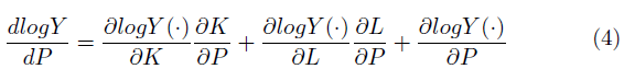
Simplifying,

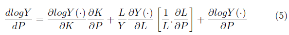
The elasticity ψ of economic output with respect to effective labour is given by;

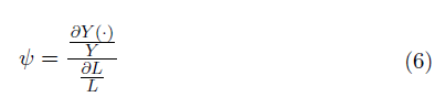
Thus, combining equations (1), (5), and (6) and simplifying, we get:

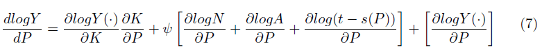
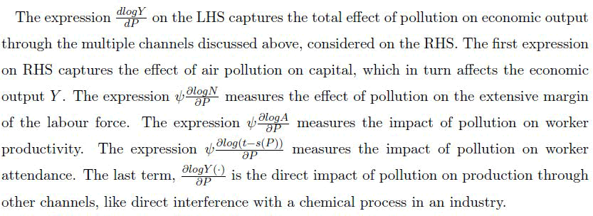
Through econometric analysis, we estimate the sign and magnitude of the expression on the LHS.

Materials and Methods

Econometric Model

The objective is to evaluate the causal effect of air pollution due to stubble burning in Punjab and Haryana on the economic output of the national capital city of New Delhi.

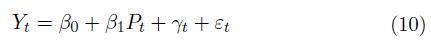
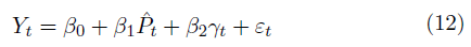
In this study, we use regression analysis with instrumental variable analysis to account for confounding effects of other variables and reverse causality. The basic econometric model that can be used to characterize the relationship between economic output and air pollution levels due to stubble burning at time t can be stated as follows:

Where:

Y_t=Variable that denotes the economic output at time t,
β₀=Captures the fixed effects of the city,
P_t=Pollution level at time t,
γ_t =Time-varying impacts on economic output in the region due other factors,
ε_t=Error term.

In this model, a few constraints need to be addressed. First is the reverse causality of increase or decrease in economic output on air pollution levels. In the past it has been observed that when pollution levels in New Delhi are very high, policy interventions cause certain businesses and schools to shut down or reduce the working hours [32] reducing pollution from industries. This further causes reduction in road traffic and air pollution from vehicular emissions as well. All of these factors contribute to lowering of air pollution levels due to ambient effects. Thus, there is a reverse causality between economic output and pollution due to local factors. This can be characterized as follows:

Economic activity ↑ ⇒ Air pollution levels ↑
Air pollution levels↑ ⇒ Economic activity ↓
Economic activity ↓ ⇒ Air pollution levels ↓

Due to this cyclical causality, a simple regression with pollution level, in spite of other controlling variables, is unlikely to give an unbiased estimate of changes in economic output. Therefore, to measure the impact of air pollution due to stubble burning, which is not a local phenomenon, we need to use a different methodology.

Instrumental Variable Analysis

To address this constraint, we use instrumental variable analysis [33]. Since the phenomenon whose causal effect we wish to estimate is the burning of crop residue in North-West India, it is ideal to take the number of field fires at time t as an instrumental variable. We call this variable as FIRECOUNT. Open field fires in north-western regions of Punjab and Haryana emit pollutants into the air, and the wind carries these pollutants to the national capital city of New Delhi. The number of fires at any given time t is a good indicator of the concentration levels of pollutants present in the air. The FIRECOUNT satisfies the requirements of an instrumental variable, namely:

• Exclusion restriction: It affects the dependent variable (economic output) only through the explanatory variable (pollution levels in New Delhi).
• It is correlated with the explanatory variable (pollution levels in New Delhi).
• It is not caused by the dependent variable (economic output of New Delhi), and is thus exogenous, and as good as randomly assigned.

FIRECOUNT, or the number of field fires in Punjab and Haryana, can be safely assumed to have no effect on the Gross State Domestic Product (GSDP) of New Delhi via any channel other than air pollution. The fires are in different states, and thus, are not correlated with or caused by economic activity in New Delhi. FIRECOUNT does have a direct correlation with the air pollution levels in New Delhi, as already found by numerous studies and satellite information. As visible in Figures 1 and 6, the variation of PM2.5 in New Delhi with time and the variation of FIRECOUNT in north-west India with time, both follow the same pattern every year, for all stations.

First stage: Since the effect of wind speed cannot be ignored on the concentration of pollutants in the air, wind speed is taken as a control variable in measuring the effect of field fires. Other control variables are meteorological parameters like Relative Humidity (RH), Wind Direction (WD) and Air Temperature (AT). Pollution levels are measured for PM2.5 or PM10.

So, the first stage of the analysis (taking wind speed as a control variable) would be:

Where:

P_t=Pollution level at time t,
α₀=Captures fixed effects,
FIRECOUNT=Total number of field fires at time t,
WS_t=Wind speed at time t (control variable),
Θ_t=Error term at time t.

Second stage: A lot of variables affect the GSDP of a city: Economic and natural shocks, changes in world economic activity, changes in population demographics etc to name a few. It is important to control for these effects so as to be able to measure the effect of pollution levels on economic output without omitted variable bias. Since a lot of data of these variables is not available for the city of New Delhi, an index which is computed considering many such effects is instead used as a control variable-the subnational Human Development Index (HDI) for New Delhi by UNDP [34]. The subnational HDI accounts for variation in changes in socio-economic structures with time γ_t. We use the Gross State Domestic Product (GSDP), GSDP per capita and Gross State Value Added (GSVA) of New Delhi as measures of economic output Y_t in the model. The second stage is thus given by:

Where:

Y_t=Economic output,
β₀=Captures fixed effects,
P_t=Pollution level at time t (as evaluated from the first stage regression),
Γ_t=Captures time-varying effects on economic output (control variable),
Ε_t=Error term.

Reduced form

We use “Two Stage Least-Squares (2SLS)” to compute the coefficient β₁. To implement this, we first estimate the first stage, and then compute the predicted values of the regressor:

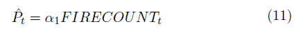
Then we regress the economic output on the predicted values of pollutant levels: In a large sample, the coefficient thus got will be β₁.

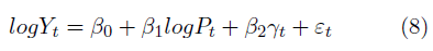
Due to a vast difference in the range of values in pollutant levels and GSDP, a log-likelihood estimation method is most appropriate for the analysis. Therefore, we instead use the log of GSDP and pollution levels as variables in the regression. Rewriting equation (12) to account for this change, we have:

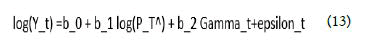
The coefficient thus obtained, b_1, gives the elasticity of economic output with respect to pollutant levels. A 1 percent increases in the levels of the pollutant causes a b_1 percent change in the economic output.

Air Pollution Data

For this study, air pollution data for nine years–from 2012 to 2021 was collected from fixed-site monitoring stations of the central and state pollution control boards in New Delhi. Data of 24 hr averages for PM2.5, PM10, CO, NO₂ and SO₂ were collected for five monitoring stations spread across the city:

Anand Vihar, ITO, Mandir Marg, Shadipur and R. K. Puram. For other monitoring stations, archival data for pollution levels was not available. Thus, these monitoring stations were selected. Since archival data of all the years for all the parameters was not available for every monitoring station, the years for which the data was available for each station was taken on a case-by-case basis. Each monitoring station records data independently of all other stations, and as such, the results from the analysis of the data of each station are independent of other stations.

A plot of the variation of pollution levels of different pollutants with time is seen in Figure 1. As stubble burning is a yearly phenomenon which takes place from September to December every year, the trend in increase in pollutant levels during this period is clearly visible in the plot. The gaps in the plot are the periods for which data for pollutant levels is not available. Time variation of PM2.5 levels for the different monitoring stations is seen in Figure 2. PM2.5 and PM10 concentrations were measured in μg/m³, CO in mg/m³, NO₂ in μg/m³ and SO₂ in mg/m³.

A correlation plot between the pollution parameters showed a high correlation between PM2.5 and PM10 values. Mild correlation was also observed between other pollutant values, as seen in Figure 2. PM2.5 was found to be the most correlated with FIRECOUNT values (Corr: 0.3), followed by PM10. Other parameters had low correlation values with FIRECOUNT, and as such, were not selected to be the endogenous variable. The data for other parameters was also found to be not as well documented as that for PM2.5 and PM10.

The relationship between FIRECOUNT and log (PM2.5) for station 1 can be seen in Figure 3. The relationship between FIRECOUNT and log (PM10) for station 4 can be seen in Figure 4.

Since PM2.5 and PM10 were found to be highly correlated, the two parameters are not used together in the regression, so as to avoid the multicollinearity effect. Instead, the two parameters are used as alternatives to measure the effect of fires on air pollutant concentrations.

Figure 1: Variation in pollutant levels across time for station.

The objective of the study is to measure the effect due to stubble burning, and PM2.5 and PM10 both can be considered to be alternative variables for that effect. For some of the stations, PM10 data is missing for several months, and as such, PM2.5 is taken as the common variable for all regressions, and PM10 is used to verify the results, where the data is available.

Crop residue fire data

To get the crop residue fire data, Active Fire Data by Visible Infrared Imaging Radiometer Suite (VIIRS) taken by Earthdata by NASA was obtained for the years 2012-2021 [3]. The data is for the region of South Asia. We take the regions where crop residue burning takes place as the region lying between the latitudes and longitudes of 28.9 N and 34 N and 73 E to 77 E respectively. The data for this region was filtered from the larger dataset. Next, the number of fires for each day was counted for this filtered region. This yields a daily count of fires in the regions of Punjab and Haryana. Data for the months of September-December was further filtered out, since those are the months of interest when crop residue is burnt. This is the data that is used in the regression analysis.

The variable FIRECOUNT gives the daily count of number of open field fires thus obtained. The yearly repeating patterns and variations in the number of field fires per day can be in Figure 6.

Figure 2: Regression of log(PM2.5) with FIRECOUNT for station 1.

Though FIRECOUNT does not reflect the intensity or extent of the field fires, the variable was found to be acceptable due to the averaging effect of small and big fires. Moreover, FIRECOUNT values vary from as low as 1 and 2 per day up to a maximum of 8000 fires per day. Due to this broad range of values, the peak season can be clearly identified in the data, usually in the months of October and November. Thus, FIRECOUNT was found to be a good variable to characterize the effect of stubble burning in the region.

Weather Data

Weather data for New Delhi is obtained from fixed-site monitoring stations of the central and state pollution control boards in New Delhi. Data for Relative Humidity (RH), Wind Speed (WS), Wind Direction (WD), Spectral Radiance (SR), Barometric Pressure (BP) and Air Temperature (AT) was compiled for 24 hr averages of values for the years (2012-2021).

Figure 3: Regression of log (PM10) and FIRECOUNT for station 4.

2012-2021. Data for the months of September-December for every year was used for the regression analysis.

On regressing PM2.5 with each of the weather variables as control variables, not much difference was found on the coefficient of FIRECOUNT. Thus, the other variables are not significantly correlated with PM2.5. The main contributor to the changes in the coefficient was Wind Speed (WS), which was found to be negatively correlated with the pollution levels. This is expected since high wind speeds cause the winds to carry away pollutants from the capital city, thus lowering the pollutant levels in the air. When wind speeds are low, pollutants stagnate in the air above the ground, mixing with the fog and dust to form a thick layer of smog above the ground, which is not only harmful for health, but also reduces visibility on the ground.

Thus, Wind Speed (WS) was found to be the ideal control variable upon preliminary evaluation of the available data.

Figure 4: Correlation plot of variables.

Economic data

The economic data for New Delhi was available as yearly values. The GSDP, GSDP per capita and GSVA values were taken from the New Delhi government portal [35], reported in INR crores at current prices. To control for variations in the economic output due to other socio-economic factors, the subnational Human Development Index (HDI) for New Delhi is used as a control variable. HDI for every year, from 2012 to 2019 is taken from the Global Data Lab website [34]. The subnational HDI was created by Global Data Lab using three sources: Statistical offices (including Eurostat, the statistical office of the European Union), the Area Database of the global data lab, and data from the HDI website of the Human Development Report Office of the United Nations Development Program. Thus, it can be considered to be a robust measure of socio-economic effects on the economy. It is reported as an index, with 0 ≤ HDI index ≤ 1.

Since pollutant concentration values will not be negative or zero, and to account for the wide range of values in pollutant concentrations and economic output, logarithm of pollutant concentration was regressed against the logarithm of economic output in the second stage regression (Figure 5).

Figure 5: PM2.5 (IN μG/M3) trend with time for the 5 stations.

As expected, the FIRECOUNT data was found to have zero correlation with the economic data of GSDP, also seen in the correlation plot in Figure 4. This further validates our assumption that the exclusion restriction for the instrumental variable holds for this study.

Data Processing and Analysis in Python

The air pollution data and weather data obtained from central and state pollution control boards is 24 hr average data for the pollutant parameters. The crop residue burning FIRECOUNT data is counted for 24 hr periods, and is thus, a total count of the number of fires in the 24 hrs on that date. The weather data follows the pattern of the air pollution data, as it is from the same source. But the weather data is not available for every monitoring station in New Delhi. Thus, the weather data is taken from a monitoring station in central part of New Delhi, and assumed to be the same throughout Delhi, taking the effects of micro-climates to be negligible. This is a reasonable assumption since the variations in meteorological data across New Delhi are small [36].

Though we take PM2.5 and PM10 as the explanatory variables for pollution, the economic cost of air pollution due to crop residue burning can well be due to other pollutants as well, and the study estimates the cost due to all the pollutants (Figure 6).

Figure 6: FIRECOUNT trend with time.

The possibility of a lag between field fires and rise in pollutant levels over New Delhi was considered. But it was found that the lag between lighting a fire in northwestern regions and the pollutants reaching the capital city is not more than 24 hours, based on the wind speed and other meteorological effects. Moreover, some of the fields are much closer to the city, whereas some of the fields are further way. On average, the fields can be considered to be within a 24 hr lag from lighting fires and rising of pollutant concentration levels in New Delhi. Thus, the effect of lag on the pollution data was taken to be negligible.

The economic data is reported by government and international organizations yearly. No data for GSDP or GSVA of Delhi could be found for any period shorter than one year. To merge this data with the rest of the data, the daily pollution, weather and FIRECOUNT data would have to be averaged yearly, or the GSDP can be taken as constant for every day in one year. Averaging the pollutant and other data would fail to capture the trends and variations in the pollutant levels with time. Averaging would remove all the variation of pollutant levels with increase and decrease in FIRECOUNT. Moreover, it would reduce the data to merely that of 9 years (six years for some of the monitoring stations for which data is not available for every year). This would not be sufficient to run a regression and arrive at results with any level of accuracy. Thus, the GSDP and HDI were instead taken as constant for every single day in a year, and the entire dataset for every monitoring station was regressed as discussed above.

We run two regressions (first stage and second stage) for each set of variables (FIRECOUNT, PM2.5, GSDP and control variables) for each of the 5 monitoring stations’ data. We then check the results by replacing PM2.5 with PM10 and see if there is a remarkable difference in values. We then again check the results by replacing GSDP with GSVA and GSDP per capita. And see if there is a remarkable difference in values reported. Thus, the reported results are a compilation of the results from 20 regressions, 4 each for the 5 monitoring stations.

Results and Discussion

The results of the first stage regression show a consistent positive correlation between FIRECOUNT and PM2.5 levels, and a negative correlation between WS and PM2.5 levels. The same trend is observed for data across all the five monitoring stations. The values of the coefficients and standard errors for all the variables and intercept fall in the same range for all the five monitoring stations. The data of each of these monitoring stations is collected by sensors independent of other sensors, and the number of observations for each station is also different. Some of the stations are missing the data for certain years or months, and as such, the time period over which the data is available and used for each station is different. Nevertheless, the results for the regression fall within an acceptable range for all coefficients, and are statistically significant at the 99.9 percent level.

The OLS for PM10 and FIRECOUNT yields similar results, with a slightly wider variation in the coefficients (than those obtained in the regression with PM2.5), but still within acceptable levels. The overall trend of all the values for all the monitoring stations is the same, and all are statistically significant at the 99.9 percent level.

The output of the first stage OLS is in keeping with the theoretical understanding of the phenomenon. The coefficients of FIRECOUNT fall in a narrow range and are statistically significant, so the predicted values of PM2.5 and PM10 levels can be taken as the pollution levels due to crop residue burning, and plugged into the second stage OLS regressions.

The second stage OLS results are in alignment with our theoretical framework to assess the impact of pollution on economic output. The coefficient for pollutant levels is negative, implying that the result of an increase in pollutant levels is a decrease in economic output. The results for the second stage regression for log (PM2.5) and log (GSDP) are statistically significant at the 99.9 percent level (Table 1-7).

Table 1: First stage OLS for PM2.5 and FIRECOUNT.

The second stage OLS regression results yield a coefficient of approximately -0.01 for log (PM2.5) as regressor for log (GSDP). This implies that a 1 percent change in PM2.5 levels would cause the GSDP to decrease by 0.01 percent. Thus, a 100 percent increase in PM2.5 levels would cause the GSDP of New Delhi to decrease by 1 percent. During the peak stubble burning season, high values of PM2.5, exceeding 500 μg/m³ are often observed. Not only is this air toxic to breathe, this value of PM2.5 concentration is almost five times or five hundred percent of the PM2.5 values during the rest of the year (also visible in the yearly variation of pollutant levels in Figure 5). As per the relationship established from the OLS results, this could cause up to 5 percent decrease in economic output of New Delhi, measured in GSDP at current prices. For context, 5 percent of the GSDP of New Delhi is approximately INR 39,915 crores (at current prices) for the year 2020-2021. This analysis is merely to illustrate how changes in air pollutant levels due to stubble burning can affect the economic output of New Delhi as per our findings. If the values of pollutants remain at high levels for long periods of time, they could potentially cause a higher decrease in GSDP in the coming years.

Table 2: First stage OLS for PM10 and FIRECOUNT.

To check the robustness of the findings, we run the second stage regression again, changing the variables. Similar results are obtained by replacing PM2.5 with PM10 and GSDP with GSVA or GSDP per capita (Tables 3-7). In each regression, the coefficients of log (PM2.5) and log (PM10 ) have a negative sign and are in the same order of magnitude for all monitoring stations. The coefficient of HDI also follows the same sign and order of magnitude in each regression for all stations. The results are statistically significant. Data from each monitoring stations is independent of all other stations; as such, each regression is an independent finding. Since the findings are consistent across all the variables, it is concluded that the results strongly suggest a negative impact of air pollution due to stubble burning on the economic output of New Delhi, and that the change in economic output corresponding to a one percent change in pollutant levels due to stubble burning is approximately -0.01 percent.

Table 3: Second stage OLS for log(PM25) and log(GSDP).

Table 4: Second stage OLS for log(PM2.5) and log(GSDP per capita).

Table 5: Second stage OLS for log(PM25) and log(GSVA).

Table 6: Second stage OLS for log(PM10) and log(GSDP).

Table 7: Second stage OLS for log(PM10) and log(GSVA).

Conclusion

The results illustrate that crop residue burning in Punjab and Haryana are negatively correlated with the GSDP of New Delhi. Thus, controlling air pollution is urgently required, not just on moral, health or environmental preservation reasons, but for economic reasons as well. This requires a policy which incentivizes the wider adoption of existing solutions that eliminate the need to burn crop residue by giving better, or more economically viable alternatives to the farmers. Enriching the soil with biochar prepared from paddy stubble is one such alternative. Other methods can be better management of labour wages and availability in these states. The state governments can directly employ workers to cut the crop residue, and take the stubble from farmers in return for the labour. The biochar produced from this stubble can then be sold to farmers all over the country at subsidized prices. Policy designs which solve the causes of stubble burning are expected to be the most effective.

For a growing economy like India, ignoring the long-run and short-run economic impacts of environmental damage can prove to be a costly mistake a few decades down the line. Immediate policies and their implementation are required to solve this growing problem, which has been left unheeded for the last two decades.

Competing Interests

No competing interests.

Funding Statement

The authors received no specific funding for this work.

Acknowledgements

The authors thank Dr Alpana Agarwal, Dr Parth Parihar and Dr Nitish Mital for their valuable suggestions and inputs to the research article.

References

1. CPCB. Central control room for air quality management-Delhi NCR. Government of India. 2017.
2. National Clean Air Programme. Technical report, ministry of forest, environment and climate change, government of India, 2019.
3. Abadie A, Cattaneo MD. Econometric methods for program evaluation. Annu Rev Econ. 2018;10:465-503.

   [Crossref] [Google Scholar]

4. Adhvaryu A, Kala N, Nyshadham A. Management and shocks to worker productivity. J Political Econ. 2022;130(1):1-47.

   [Crossref] [Google Scholar]

5. Ali N, Islam F. The effects of air pollution on COVID-19 infection and mortality. A review on recent evidence. Front Public Health. 2020;8:580057.

   [Crossref] [Google Scholar] [PubMed]

6. Dechezlepretre A, Rivers N, Stadler B. The economic cost of air pollution: Evidence from Europe. OECD Economics Department Working Papers, No. 1584, OECD Publishing, Paris. 2019;62.

   [Crossref]

7. Aragon FM, Miranda JJ, Oliva P. Particulate matter and labor supply: The role of caregiving and non-linearities. J Environ Econ Manage. 2017;86:295-309.

   [Crossref] [Google Scholar]

8. Balakrishnan K, Ganguli B, Ghosh S, Sankar S, Thanasekaraan V, Rayudu VN, et al. Part 1. Short-term effects of air pollution on mortality: Results from a time-series analysis in Chennai, India. Res Rep Health Eff Inst. 2011;1(157):7-44.

   [Google Scholar] [PubMed]

9. Bashir MF, Jiang B, Komal B, Bashir MA, Farooq TH, Iqbal N, Bashir M. Correlation between environmental pollution indicators and COVID-19 pandemic: A brief study in Californian context. Environ Res. 2020;187:109652.

   [Crossref] [Google Scholar] [PubMed]

10. Beig G, Sahu SK, Singh V, Tikle S, Sobhana SB, Gargeva P, et al. Objective evaluation of stubble emission of North India and quantifying its impact on air quality of Delhi. Sci Total Environ. 2020;709:136126.

    [Crossref] [Google Scholar] [PubMed]

11. Bherwani H, Nair M, Musugu K, Gautam S, Gupta A, Kapley A, Kumar R. Valuation of air pollution externalities: Comparative assessment of economic damage and emission reduction under COVID-19 lockdown. Air Qual Atmos Health. 2020;13:683-694.

    [Crossref] [Google Scholar] [PubMed]

12. Cusworth DH, Mickley LJ, Sulprizio MP, Liu T, Marlier ME, DeFries RS, et al. Quantifying the influence of agricultural fires in northwest India on urban air pollution in Delhi, India. Environ Res Lett. 2018;13(4):044018.

    [Google Scholar]

13. Global Data Lab. Subnational HDI (v5.0). Institute for Management Research, Radboud University, 2013-2023.
14. Hansen-Lewis J. Does air pollution lower productivity. Evidence from Manufacturing in India. 2018;56.

    [Google Scholar]

15. Khare P, Deshmukh Y, Yadav V, Pandey V, Singh A, Verma K. Biochar production: A sustainable solution for crop residue burning and related environmental issues. Environ Prog Sustain Energy. 2021;40(2):e13529.

    [Crossref] [Google Scholar]

16. Gopi C, Khilnani, Tiwari P. Air pollution in India and related adverse respiratory health effects: Past, present, and future directions. Curr Opin Pulm Med. 2008;24(2):108-116.

    [Crossref] [Google Scholar] [PubMed]

17. Kumar A, Kushwaha KK, Singh S, Shivay YS, Meena MC, Nain L. Effect of paddy straw burning on soil microbial dynamics in sandy loam soil of Indo-Gangetic plains. Environ Technol Innov. 2019;16:100469.

    [Crossref] [Google Scholar]

18. Lohan SK, Jat HS, Yadav AK, Sidhu HS, Jat ML, Choudhary M, et al. Sharma PC. Burning issues of paddy residue management in north-west states of India. Renew Sust Energ Rev. 2018;81:693-706.

    [Crossref] [Google Scholar]

19. Maji K, Dikshit AK, Deshpande A. Assessment of city level human health impact and corresponding monetary cost burden due to air pollution in India taking Agra as a model city. Aerosol Air Qual Res. 2017;17(3):831-842.

    [Crossref] [Google Scholar] [PubMed]

20. Panteli M, Delipalla S. The economic cost of ill health due to air pollution: Evidence from Greece. Int J Appl Bus Econ Res. 2021.

    [Google Scholar]

21. Borgschulte M, Molitor D, Zou E. Smoked out: The effect of wildfire smoke on labor market outcomes. Technical report, technical report. Working Paper; 2016.

    [Google Scholar]

22. Ministry of Statistics and Programme Implementation. Economy of Delhi, 2021.
23. Mohr RD. Technical change, external economies, and the Porter hypothesis. J Environ Econ Manage. 2002;43(1):158-168.

    [Crossref] [Google Scholar]

24. NASA. Active Fire Data. Fire Information for Resource Management System, 2023.
25. Pandey A, Brauer M, Cropper ML, Balakrishnan K, Mathur P, Dey S, et al. Health and economic impact of air pollution in the states of India: The global burden of disease study 2019. Lancet Planet Health. 2021;5(1):e25-38.

    [Crossref] [Google Scholar] [PubMed]

26. Porter ME. Competitive advantage of nations: Creating and sustaining superior performance. Simon and Schuster; Free Press, 2011:896.

    [Google Scholar]

27. Quah E, Boon TL. The economic cost of particulate air pollution on health in Singapore. J Asian Econ. 2003;14(1):73-90.

    [Crossref] [Google Scholar]

28. Rajput P, Gupta T. Instrumental variable analysis in atmospheric and aerosol chemistry. Front Environ Sci. 2020;8:566136.

    [Crossref] [Google Scholar]

29. Sangwan V, Deswal S. In-situ management of paddy stubble through microbial biodegradation. InE3S Web of Conferences, 10 March 2021, India,241: 03001.

    [Crossref] [Google Scholar]

30. Sanjay, Swamy HM, Seidu M, Singh SB. Issues of paddy stubble burning in Haryana: Current perspective. Paddy Water Environ. 2021;19:55-69.

    [Crossref] [Google Scholar]

31. Sarkar S, Singh RP, Chauhan A. Increasing health threat to greater parts of India due to crop residue burning. Lancet Planet Health. 2018;2(8):e327-e328.

    [Crossref] [Google Scholar] [PubMed]

32. Siddique S, Ray MR, Lahiri T. Effects of air pollution on the respiratory health of children: A study in the capital city of India. Air Qual Atmos Health. 2011;4(2):95-102.

    [Crossref] [Google Scholar] [PubMed]

33. Solow RM. The economics of resources or the resources of economics. In Classic papers in natural resource economics, London: Palgrave Macmillan UK,1974;257-276.

    [Crossref] [Google Scholar]

34. The Lancet Planetary Health. Government indifference over air pollution crisis in Delhi. Technical Report 9, 12 2017.

    [Google Scholar]

35. Upadhyay A, Dey S, Chowdhury S, Goyal P. Expected health benefits from mitigation of emissions from major anthropogenic PM 2. 5 sources in India: Statistics at state level. Environ Pollut. 2018;242:1817-1826.

    [Crossref] [Google Scholar] [PubMed]

36. Wang Z, Wei W, Zheng F. Effects of industrial air pollution on the technical efficiency of agricultural production: Evidence from China. Environ Impact Assess Rev. 2020;83:106407.

    [Crossref] [Google Scholar]