Journal of Pollution Effects & Control
Open Access
ISSN: 2375-4397
ISSN: 2375-4397
Research Article - (2016) Volume 4, Issue 4
Deaths resulting from CO poisoning has been a recurrent incidence in the city of Port Harcourt especially from risky behaviors, such as improper placement of power generating sets and indoor use of charcoal grills. Domestic CO poisoning is rarely reported and remains an under recognized problem. This study therefore examined the concentration of Carbon Monoxide (CO) as influenced by both landuse and meteorological parameters of wind speed, relative humidity, ambient temperature and rainfall in the industrial city of Port Harcourt. Air quality and meteorological data were measured at twelve stations: two each from the industrial, high and low density residential, commercial, transportation and surrounding rural areas. Data were collected for seven weeks during wet, transition and dry seasons. Analysis of data was done using ANOVA and stepwise multiple regression techniques. Result showed that during the wet season, wind speed was significant at 99% in impacting the concentration of CO at the low density residential areas of GRA and Abuloma housing estates. The coefficient of determination value (22.9%) showed that jointly, the meteorological variable accounted for 23.9% of the variation in the concentration of CO during the wet season at the low density residential areas. At the rural areas, the correlation matrix shows that both rainfall (-0.117) and wind speed (-0.318) correlated inversely with CO during the wet season. But air temperature (0.005) and relative humidity (0.268) correlated directly with CO. Generally, the mean weekly concentration of CO revealed that the industrial areas accounted for 28.8%, 26.7% and 22.1% of the total atmospheric loading of CO during the transition, dry and wet season respectively. Further studies are needed to link exposure to CO with mortality and morbidity.
Keywords: Mortality; Morbidity; Carbon monoxide; Meteorological parameters; Land use
The quality of indoor air is impacted by various contaminants from indoor and outdoor sources. According to World Health Organization (WHO), nearly 2 million people a year die prematurely from illnesses attributable to indoor air pollution. Among these deaths, 44% are due to pneumonia, 54% from chronic obstructive pulmonary disease (COPD), and 2% from lung cancer [1]. Therefore, this risk factor is the second largest environmental contributor to ill health, behind unsafe water and sanitation [2]. Carbon Monoxide (CO) poisoning is a leading cause of unintentional poisoning deaths around the globe [3]. CO is an odorless, colorless gas that usually remains undetectable until exposure results in injury or death. Although CO poisoning is preventable, unintentional, non-fire-related CO poisoning is responsible for approximately 15,000 emergency department visits and nearly 500 deaths annually in the United States [4]. Several population–based studies have established a strong correlation between exposures to CO ranging from 0.5 ppm to 10 ppm and increasing adverse cardiovascular outcomes, asthma symptoms, asthma severity, hospital admission rates, and heart rate among children. These values correspond to approximate steady–state blood COHb levels of <2% for the mean and <10% for the maximum [5-8]. A large body of epidemiologic studies has provided evidence that exposure to low concentrations of CO for a long period may affect learning, manual dexterity, driving performance, and attention level [9-11]. In addition to common syndromes that children may experience due to exposure to low concentrations of CO for a long period, such as headaches dizziness, nausea (feeling sick) and tiredness, CO may affect the residents’ ability to concentrate and think clearly [11-13]. Seasonal variation is considered one of the main reasons that may increase CO concentrations and consequently increase the burden of disease. Different factors, such as outdoor air concentration, meteorological factors, and human activity, may influence seasonal variation of indoor and outdoor CO concentration. Studies on the importance of meteorological parameters in determining the evapotranspiration, crop yield among others using models abound in the literature. For example, Khoshravesh et al. [14] estimated the monthly reference evapotranspiration using three different regression models which includes the multivariate fractional polynomial (MFP), robust regression, and Bayesian regression. The results show that at a monthly scale, all models provided a closer agreement between Food and Agriculture Organization (FAO) and Penman–Monteith. Valipour [15] compare mass transfer-based models to determine the best model under different weather conditions. The results showed that the Penman model estimates reference crop evapotranspiration better than other models in most provinces of Iran. Similarly, Valipour and Eslamian [16] estimated evapotranspiration using using 11 temperature-based models and was compared with the FAO Penman-Monteith model. The results showed that the modified Hargreaves-Samani models estimated the evapotranspiration better than the other models in the most provinces of Iran. Similar studies include Valipour [17-19].
The annual average outdoor CO concentrations worldwide are roughly 0.12 ppm in the Northern Hemisphere and about 0.04 ppm in the Southern Hemisphere [8]. However, the outdoor CO concentration varies from season to season, with seasonal maximum levels occurring during late winter in both hemispheres and minimum levels being observed during late summer [8]. The fluctuation of meteorological factors, such as temperature, humidity, pressure, and wind speed, through the course of the year affect CO dispersion and destruction processes by photochemical reactions over a period of months [11,20]. Reports of deaths resulting from CO poisoning has been a recurrent incidence in the city of Port Harcourt especially from risky behaviors, such as improper placement of power generating sets and indoor use of charcoal grills [21,22].
Domestic carbon monoxide poisoning is rarely reported in Port Harcourt and remains an under recognized problem [23]. The diagnosis of carbon monoxide poisoning is usually based on autopsy findings, circumstantial evidence and estimation of carboxy-haemoglobin in blood [24]. No known study has examined the influence of meteorological parameters on the behavior of CO in the city of Port Harcourt. This is the gap in the literature which this study intends to fill.
The collection of CO concentration data
Air quality and meteorological data were measured at twelve locations: two each from the industrial, high and low density residential areas, commercial, transport and rural areas (30 km away from the city). The collection of air quality and meteorological data for this study covered the period 2nd August to 18th September, 2010 reflecting the wet season; October 4th to November 20th, 2010 for the transition period and January 3rd to February 19th 2011 reflecting the dry season period. This covered about 126 days (42 days each of each three seasons). The choice of these seasons was based on rainfall distribution of Port Harcourt. The transition period of rainfall represents the period when rainfall begins to recede giving way to the dry season. It is also a period between the wet season and the dry season. This sampling framework was adopted to capture the potential fluctuations in carbon monoxide concentrations in all the stations for all the seasons. In order to select the sampling sites for air quality monitoring, a land use map of the study area with the scale 1:1,000 was converted into a gridded map of 500 m×500 m. All the cells of the gridded map were coded by their respective land use type and used to obtain two monitoring stations representing a specific landuse for all twelve stations. The spatial variations in CO concentration in this study were evaluated by analyzing the actively sampled CO data from the different land use areas chosen in this study on daily basis. The analysis was based on the data collected throughout the seasons considered in this study. The objective was to ascertain and/or identify the mean weekly spatial variations in the concentration of CO at the respective land use areas. The seasonal variation in CO concentration was done amongst the landuse types to determine the difference in the concentration of CO at different seasons of the year. Table 1 shows the geographical coordinates of the areas which constitute the major land use areas used for the study. The data was analysed using twoway Analysis of Variance and Stepwise Multiple Regression (SMR) technique with the aid of SPSS statistical software. For all the land use types, effort was made to identify the general wind direction. This was to enable us identify the down-wind and up-wind direction to enhance the quality and reliability of the data that was collected.
| Landuse | Stations | Latitudes (°N) | Longitudes (°E) |
|---|---|---|---|
| Industrial | Eleme | 4°47' | 7°6' |
| Trans-Amadi | 4°48' | 7°1' | |
| High density residential | Diobu | 4°47' | 6°59' |
| Rumuagholu | 4°52' | 6°59' | |
| Low density residential | GRA | 4°48' | 6°59' |
| Abuloma housing estate | 4°46' | 7°2' | |
| Commercial | Mile III Market | 4°48' | 6°59' |
| Creek road market | 4°45' | 7°1' | |
| Transport | PH-Aba exprees way | 4°48' | 7°0' |
| Ikwerre road | 4°52' | 6°59' | |
| PH Int’l Airport | 5°0' | 6°57' | |
| Rural | Aluu | 4°56' | 6°56' |
| Egbelu-akami | 4°50' | 6°57' |
Table 1: Geographical coordinates of sampled stations.
The relationship between weather parameters and CO concentration at the sampled points were examined using the Multiple Linear Regression (MLR) analysis. The CO concentration was the dependent variable and the other atmospheric parameters were the independent variables. This enabled us to identify the degree and nature of the relationship between the climatic parameters and CO concentrations in the city. The multiple regression technique is of the form;
Y = a+ β1 x1 + β2x2 + β3x3…+ βiji + e (1)
Where,
Y = Pollutant concentration
a = Constant term
β1 β2 β3 …βJ = Regression coefficients
X1 X2 X3 ...XJ = Independent variables (air temperature, wind speed and relative humidity)
The application of GIS in generating land use - CO concentration maps
Geo spatial data processing and analysis: Landsat Enhanced Thematic Mapper Plus (ETM+) image of 2007 covering the four LGAs (i.e. Eleme, Obi/Akpor, Port Harcourt and Ikwerre) was obtained for this study. The Landsat ETM+ satellite data was processed using ERDAS IMAGINE 9.2 image processing software. The image was imported into ERDAS using ERDAS native file format GEOTIFF. Since the images were in single bands, they were stacked together using ERDAS layer stack module to form a floating scene and to group the bands together. The 2007 image was co-registered with other images and later geo-linked to allow for the subset of the image to the study area. This was followed by performing further Geometric corrections of the 2007 image to remove few scattered clouds in the image. The image was projected to the Universal Traverse Mercator (UTM) coordinates zone 32. The spheroid and datum was also referenced to WSG84. Enhancement of the images using histogram equalization techniques was later performed on the image and subset to an area to cover the four LGA. The image was later displayed as false-color composites with band combination of red as band 4, green as band 3, and blue as band 2. All the images were later categorized using supervised classification technique to identify land cover features within the study area.
The supervised classification was done by defining the number of classes to be 10 depending on the number of possible classes that can be readily identified by the software. Names were later assigned to the classes based on the patterns that could be identified. The classified map was later imported into ArcGIS 9.2 software for preparation and production.
Contour creation and data preparation: The following steps were taken to prepare the data.
1. The XY data i.e. the sample points obtained from the field was prepared in Excel Spread Sheet and saved in a format recognized by ArcGIS.
2. The Points were plotted in ArcGIS by the use of the ADD XY data module found in the Tool Menu of ArcGIS 9.2 software.
3. An Attribute database was created for the sample points during which all the values obtained from the field were keyed into their respective sampled stations field or Row and Columns.
Data analysis
The Spatial Analyst Tool in the ArcToolBox was used to analyze the data obtained from the field after its preparation so as to meet the necessary conditions that permit its analysis in ArcGIS. Two tools were used, one is the SPLINE tool for data Interpolation found in the Spatial Analyst and the second is the CONTOUR tool present in the Surface analysis Box for carrying out surface analysis such as Contours, Aspect, and Slope etc. The contour maps were created from the SPLINE data generated from the sample points and the CO concentration for the different seasons (wet, transition and dry seasons). The Produced contour maps were later superimposed on the landuse map generated earlier. Labeling of the contour values and the sample stations were done and the map was taken to layout view for preparation and production. The produced maps were finally exported and saved in jpegs for easy accessibility to word document.
Spatial and seasonal concentration of carbon monoxide
The variation in the mean weekly concentration of CO as shown in Figure 1 revealed that during the transition period on the first week of measurement across the entire land use areas, Carbon Monoxide values were highest at the industrial areas with a peak mean value of 36.15 mg/ m3. This was followed by the transportation land use area with a mean value of 31.48 mg/m3. The variation in the mean weekly concentration of CO progressively decreased from the high density residential area (25.40 mg/m3) to the commercial land use area (22.85 mg/m3); rural land use (22.42 mg/m3) to its lowest value at the low density residential area (1948 mg/m3) The mean weekly concentration of CO during the dry season was highest at the industrial area (130.37 mg/m3); this value progressively reduced from transportation (38.6 mg/m3); HDR (32.72 mg/m3); rural (41.11 mg/m3); LDR (47.57 mg/m3;) to its lowest in the commercial area (18.92 mg/m3). The mean weekly CO concentration for the different landuse types during the wet season were as follows: transportation (21.7 mg/m3); HDR (14.8 mg/m3); industrial (10.17 mg/ m3) rural (9.2 mg/m3) and commercial (7.1 mg/m3).
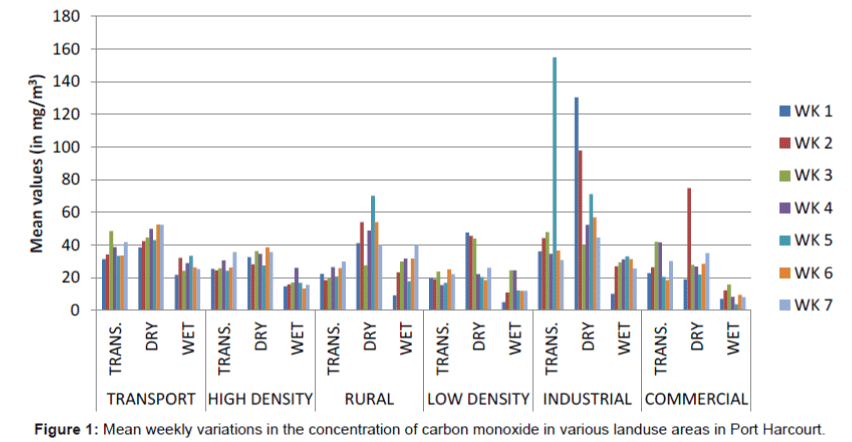
Figure 1: Mean weekly variations in the concentration of carbon monoxide in various landuse areas in Port Harcourt.
The summary of the concentration of CO for the rest of the six weeks showed that the industrial area (97.72 mg/m3) had the highest value during the dry in the second week. But in the third week, commercial area (48.49 mg/m3) has its peak during the transition period. Similarly, the industrial area (52.3 mg/m3) had the highest concentration of CO on the fourth week which progressively reduced from transportation (49.86 mg/m3); rural (48.77 mg/m3); HDR (34.64 mg/m3); Commercial (26.81 mg/m3) and LDR (22.28 mg/m3) for the same dry season. During the fifth week, concentration of CO continued to increase at the industrial area (71.18 mg/m3) and decreased progressively to the rural (70.04 mg/m3) transportation (43 mg/m3), HDR (27.49 mg/ m3), Commercial (22 mg/m3) and LDR (20.48 mg/m3) during the dry season. In the sixth week, the industrial area had a high concentration (56.99 mg/m3) which decreased gradually in the rural (53.93 mg/ m3), transportation (52.43 mg/m3), HDR (38.54 mg/m3), commercial (28.51 mg/m3) and LDR (18.64 mg/m3) during the dry season. The mean weekly concentration of CO was similarly high at the industrial (44.57 mg/m3) and reduced accordingly at the transportation (41.82 mg/m3), rural (40.16 mg/m3), HDR (35.64 mg/m3), commercial (34.98 mg/m3) and LDR (25.97 mg/m3 during the dry season in the seventh week. Generally, the mean weekly concentration of CO revealed that the industrial areas accounted for 28.8%, 26.7% and 22.1% of the total atmospheric loading of Carbon Monoxide during the transition, dry and wet season respectively in the city of Port Harcourt. This is followed by the transport area accounting for 19.4%, 17.5%, and 22.6% during the transition, dry and wet season respectively. Commercial areas accounted for 14.9%, 12.7%, and 7.6% of atmospheric loading of CO during the transition, dry and wet season respectively. The high density residential areas accounted for 14.3%, 12.7%, and 22.6% during the transition, dry and wet season respectively. The rural areas accounted for, 12.1%, 18.2% and 21.6% during the transition, dry and wet season respectively. And the low density residential areas of GRA and Abuloma Housing Estate accounted for 10.5%, 12.8% and 11.9% of the total weekly concentration of CO in the city during the transition, dry and wet seasons respectively. The study further revealed that the total amount of Carbon Monoxide emitted into the atmosphere of Port Harcourt by all the land use area investigated throughout the seasons was 4,039.57 mg/m3. The seasonal breakdown of this Figure 2 revealed that the dry season accounted for the highest value of 1843.47 mg/ m3, transition period accounted for 1346.81 mg/m3 and wet season accounted for 849.29 mg/m3. The bar graph (Figure 3) below showed the summary of the fluctuations in the mean weekly concentration of CO in all the landuse areas and season investigated.
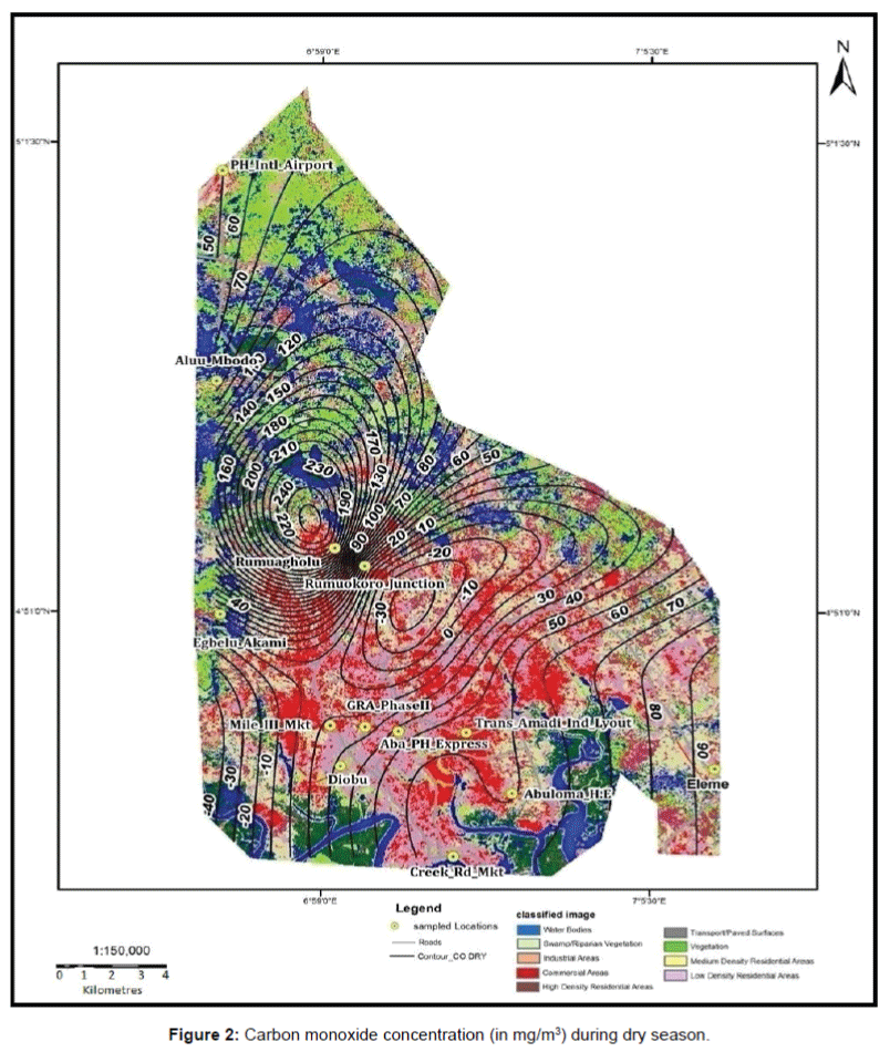
Figure 2: Carbon monoxide concentration (in mg/m3) during dry season.
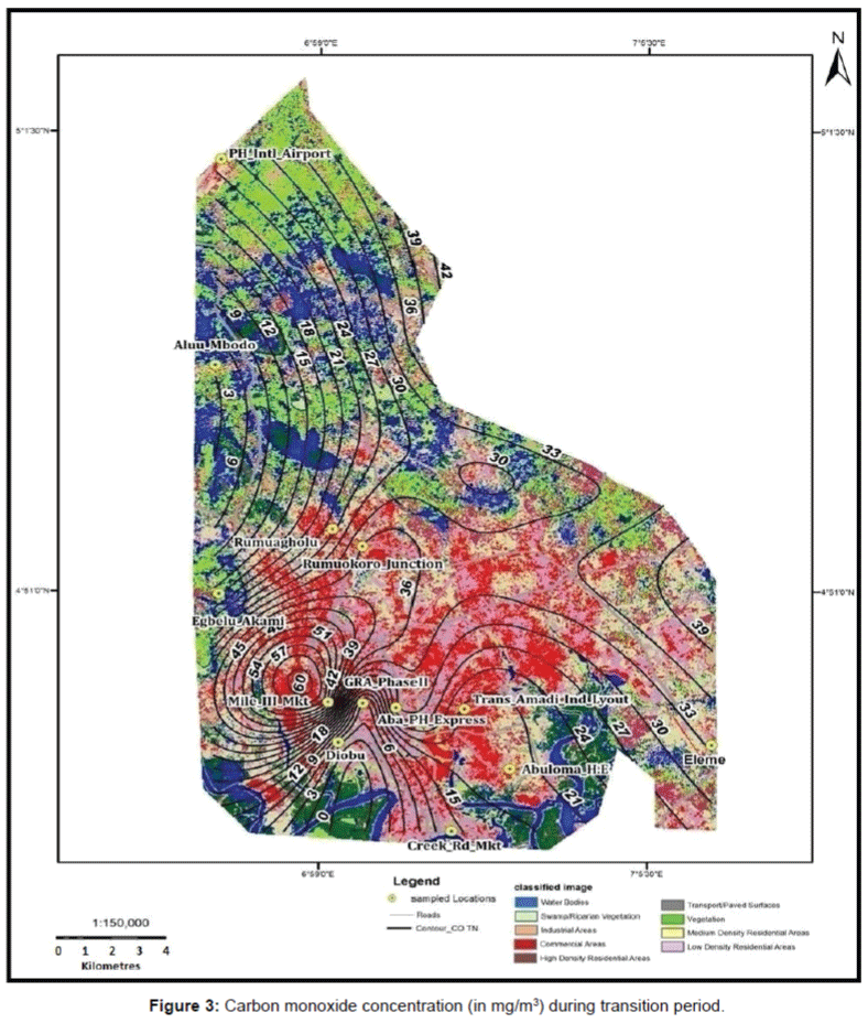
Figure 3: Carbon monoxide concentration (in mg/m3) during transition period.
The ANOVA in Table 2 decomposes the variance of CO among the various landuse areas and season into two components: a betweengroup component and a within-group component. Since the F-calculate values of 22.29, 2.92, and 4.51 for the wet, transition and dry season respectively, are greater than the F-crit. value of 2.25, we therefore conclude that “there is a statistically significant spatial weekly variation in the concentration of CO at the various landuse areas of the city at the 95% confidence level in all the seasons.
| POLLUTANT | SEASON | F.cal | F.crit | Level of significant |
|---|---|---|---|---|
| CO | Wet | 22.29 | 2.25 | Significant |
| Transition | 2.92 | 2.25 | Significant | |
| Dry | 4.51 | 2.25 | Significant |
Significant at 95% level.
Table 2: Summary of ANOVA of CO concentration amongst the various landuse areas during the wet, transition.
The relationship between carbon monoxide concentration and meteorological parameters in various landuse areas
The model result was produced for the transport, commercial low density residential and rural areas during dry, wet and dry wet and wet respectively. The correlation matrix of carbon monoxide and the meteorological variables revealed that both temperature (-0.29) and wind speed (-0.18) related inversely to the concentration of CO during the dry season. However, rainfall (0.29) and relative humidity (0.35) had direct relationship with the concentration of CO at the transport land use areas of Port Harcourt. The r2 statistics shown in Table 2, revealed that relative humidity with F-calculated values of 5.57 was significant in impacting on the concentration of CO at 95% significant level. The coefficient of determination value of 12.2% revealed that jointly, the meteorological variables accounted for 12.2% of the variations in the concentration of carbon monoxide during the dry season. At the commercial land use areas, the correlation matrix showed that during the wet season, the values of temperature (-0.06) rainfall and (-0.42) and relative humidity (-0.34) were high enough that they related inversely to the concentration of CO and only wind speed (0.049) was very low to enhance the spread of concentrated CO at the commercial areas of Port Harcourt. However, during the dry season, only rainfall values (-0.095) and relative humidity values (-0.198) correlated inversely to CO concentration and air temperature (0.044) and wind speed (0.308) related directly to CO concentration. For both wet and dry seasons, the r2 statistics shown in Table 2 revealed that relative humidity and wind speed where significant in influencing the concentration of CO at 95% significant level respectively (Figure 4). The coefficient of determination values showed that the meteorological variables jointly accounted for 11.5% and 9.5% of the variation in the concentration of CO during the wet and dry seasons respectively. At the low density residential areas, the regression model was only produced during the wet season, the correlation matrix show that rainfall (-0.15) related inversely to the concentration of CO while air temperature (0.18), wind speed (0.48) and relative humidity (0.01) related directly to CO concentration.
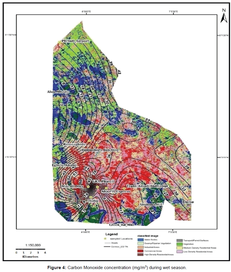
Figure 4: Carbon Monoxide concentration (mg/m3) during wet season.
The r2 statistics indicates that during the wet season, wind speed was significant at 99% in impacting on the concentration of CO at the low density residential areas of GRA and Abuloma housing estates sampled for this study (Table 3). The coefficient of determination value (22.9%) showed that jointly, the meteorological variable accounted for 23.9% of the variation in the concentration of CO during the wet season at the low density residential areas. At the rural areas, the correlation matrix shows that both rainfall (-0.117) and wind speed (-0.318) correlated inversely to the concentration of CO during the wet season. But air temperature (0.005) and relative humidity (0.268) related directly to the concentration of CO. This implies that as rainfall and wind speed increases, the concentration of CO decreases during the wet season. But air temperature and relative humidity values were very low that they indeed the concentration of CO at the areas. It was discovered that wind speed was significant at 99% significant level in determining the concentration of CO at the rural areas. Secondly, the coefficient of determination values (10.1%) show that jointly the meteorological variables accounted for 10.1% of the variations in the concentration of CO during the wet season at the rural areas sampled for this study. The predictive models for the concentration of CO as influenced by the meteorological variables are shown in Table 4. The GIS based maps of landuse and CO concentrations at different seasons are shown.
| Landuse | Season | r | r2 | F | P-values | Critical F-values | Variables in the equation | SSE |
|---|---|---|---|---|---|---|---|---|
| Transport | Wet | - | - | - | - | - | - | - |
| Transition | - | - | - | - | - | - | - | |
| Dry | 0.350 | 0.122 | 5.576 | 0.023 | 4.08 | CO/RHUM* | 10.32 | |
| Industrial | Wet | - | - | - | - | - | - | - |
| Transition | - | - | - | - | - | - | - | |
| Dry | - | - | - | - | - | - | - | |
| Commercial | Wet | 0.340 | 0.115 | 5.214 | 0.028 | 4.08 | CO/RHUM* | 138.96 |
| Transition | - | - | - | - | - | - | - | |
| Dry | 0.308 | 0.095 | 4.197 | 0.047 | 4.08 | CO/WS* | 41.72 | |
| High density residential | Wet | - | - | - | - | - | - | - |
| Transition | - | - | - | - | - | - | - | |
| Dry | - | - | - | - | - | - | - | |
| Low density residential | Wet | 0.489 | 0.239 | 12.549 | 0.001 | 7.31 | CO/WS** | 9.33 |
| Transition | - | - | - | - | - | - | - | |
| Dry | - | - | - | - | - | - | - | |
| Rural | Wet | 0.318 | 0.101 | 4.514 | 0.040 | 4.08 | CO/WS* | 14.05 |
| Transition | - | - | - | - | - | - | - | |
| Dry | - | - | - | - | - | - | - |
*Significant at 95%, ** Significant at 99%, - No Variance and /or Pollutant not detected, RHUM-Relative humidity; WS-Wind speed; TEMPT-Temperature; RFALL-Rainfall.
Table 3: r2 Statistics for CO Concentration during the wet, transition and dry Season.
| Model S/N |
Landuse | Prediction Model |
|---|---|---|
| 1 | Transport (Wet) | CO Conc.= 8.042 + 0.817 (RHUM)+ 10.32 |
| 2. | Commercial (Wet) | CO Conc. = 529.951 – 7.341(RHUM)+ 138.96 |
| 3 | Commercial (Dry) | CO Conc. = -2.866 + 61.233(WS) + 41.72 |
| 4 | Low density residential (Wet) | CO Conc.= 7.662 + 8.030(WS) + 9.33 |
| 5 | Rural (Wet) | CO Conc.= 42.018 – 17.175(WS) + 14.05 |
Table 4: Predictive Model Summary for CO in Port Harcourt.
The study has revealed that elevated carbon monoxide concentration was high at the commercial areas of Creek road and Mile III market in addition to the inhabitant of the high density residential areas of Diobu and Rumuagholu. Similarly, the high density residential areas of Nkpogu,Woji, Elenlewo, Aleto, Alesa, Ogonigba and Rumuomasi has the potential to experience an increased atmospheric temperature rise when compared to the low density residential area of GRA and Abuloma Housing Estate. It is expected that urban heat Island phenomenon will be experienced more around the residential areas sandwiched between the industrial areas, commercial and high density residential areas of the city of Port Harcourt.
CO exposures can be prevented by
1. Placing generators as far from homes as possible, but also at a safe distance from any nearby dwellings; the recommended distance for generator placement outside a home is a minimum of 25 feet (7.6 m) (3).
2. never using a generator, grill, camp stove, or other gasoline or charcoal-burning device inside a home, basement, garage, or outside near an open window.
3. Never heating homes with a gas oven or by burning charcoal.
4. Ensuring that fuel-burning space heaters are properly vented.
5. Installing a battery-operated or battery back-up CO alarm in the home.