Journal of Stock & Forex Trading
Open Access
ISSN: 2168-9458
ISSN: 2168-9458
Research Article - (2015) Volume 4, Issue 1
Option market prices have often been regarded as a window on investor sentiment about the future price behaviour of the underlying asset. Such market prices can be different than their corresponding model prices, a phenomenon revealed by implied volatility plots exhibiting “smiles” or “smirks”. Using the unique capabilities of Bayesian-based empirical methods, a four-moment risk-neutral specification is determined that largely eliminates market and model price differences. The risk-neutral density derived for a sample of S&P 500 call option prices during 2008-2009 uncovers significant market under-pricing reinforced by anomalous volatility skews that reveal bearish investor sentiment clearly signalling the pending equity market collapse
<Keywords: S&P 500 call options; Skewness; Kurtosis; Implied riskneutral distribution; Markov chain Monte Carlo; Implied volatility
The seminal work of Black and Scholes [1], henceforth abbreviated B/S, established an effective pricing mechanism for contingent-claim securities based on assumed log normally distributed security returns. However, implied volatilities or IV’s systematically greater than their corresponding B/S volatilities for a cross-section of call options of similar maturity result in the well-known volatility “smile” or “smirk”1 that raises serious questions about the validity of the distributional assumptions underlying the B/S model. For example, the “crash-ophobia” phenomenon (Rubinstein [2]; Foresi and Wu [3]) alludes to the strong demand for out-of-the-money or OTM put options on the S&P 500 index to hedge against market crashes, resulting in price increases seen as implied volatility “smirks”. Bates [4] looking at the 1987 market crash, states that OTM S&P 500 puts as crash insurance vehicles were unusually expensive relative to OTM calls. This high price could not be explained by standard option pricing models with positively skewed distributions, such as B/S, constant elasticity of variance or GARCH.
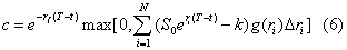
If option prices reflect investor expectations of future market performance, then the possibility arises of option market prices that are both greater than and less than their corresponding B/S prices, not just greater than B/S prices as implied by volatility “smiles” or “smirks”. Put another way, the expensive OTM S&P 500 put options used to hedge market crashes as discussed above should have call option counterparts, i.e., in-the-money (ITM) S&P 500 calls having the same strike prices, that are unusually cheap relative to B/S prices reflecting an expected decline in the future market price of the underlying asset2. In the historical graph of S&P 500 index levels shown in Figure 1 for the five-year period from 2008 through 2012, the question is whether S&P 500 call option market prices during mid-2008 signalled the extended steep decline in the index level that began in the fall of 2008? Among the reasons contributing to such poor market performance were the Lehman Brothers chapter 11 bankruptcy filing on September 15th, the buyout of Merrill Lynch by Bank of America that same September, the lending of $85 billion to AIG on September 17th, and Fannie Mae and Freddie Mac being put into conservatorship on September 7th. The S&P 500 later hit a bottom during the first half of 2009, recovered slightly, but remained low through the remainder of 2009. Such index price behaviour might be signalled by greatly reduced call option market prices for observation dates just prior to fall, 2008, relative to corresponding model prices utilizing only historical price data. Model prices that closely approximate the low market prices result from an overall decrease in implied or forward-looking return volatility relative to that derived only from past returns, resulting in IV plots lying below the constant B/S standard deviation that may not exhibit familiar IV “smiles” or “smirks”. Additionally, the components of such implied risk-neutral return volatility, specifically the implied higher moments of scale, skewness and kurtosis, can signal investor sentiment causing such anomalous price behaviour.

Figure 1: S&P 500 index level for January, 2008, through December, 2012.
Determining these higher moments requires finding the ex-ante or implied risk-neutral return probability density functions (pdf’s) that provide call option model prices closely approximating corresponding market prices. I do this for the S&P 500 market index by first estimating the model’s likelihood function based on historical index return data, then determine the ex post or historical risk-neutral pdf by adjusting its location parameter and then proceed to the ex-ante or implied version by the additional incorporation of forward-looking S&P 500 call option market prices to adjust the higher moments of scale, skewness and kurtosis to determine their implied counterparts. The critical starting point is estimation of the ex post or data-based likelihood function using Bayesian-based Markov chain Monte Carlo (MCMC) methods which offer a unique and valuable capability. MCMC output giving the marginal posterior distributions of each of the pdf’s four moment parameters as a large number of draws or iterates from such distributions are conditional only on the data. Each higher moment of scale, skewness and kurtosis defining overall return volatility is independent and, thus, such overall volatility is effectively partitioned among these three higher moments. Once the first moment of location, i.e., the mode, is found relative to the risk-free interest rate, the soughtafter ex ante or implied risk-neutral specification is that density having specific higher moment values found from MCMC output that minimizes the difference between model and market prices. These specific implied higher moment values offer a unique perspective on investor sentiment about future market performance.
Previous work by, for example, Dennis and Mayhew [6], Bollen and Whaley [7], Garleanu et al. [8] and Friesen et al. [9] document the role played by the trading activity of informed investors in influencing only the type and extent of implied skewness that leads to acceptable prediction of upcoming information events. The three implied higher moments in this paper, by effectively partitioning overall implied or risk-neutral volatility, extends our ability to more effectively reveal investor sentiment by considering each higher moment’s independent contribution to such volatility.
Comparison of the ex post physical and the ex-ante return densities reveal distinct differences between the two driven mainly by increased skewness as the 2008-2009 equity market collapse approached, resulting in familiar IV “smirks”. However, by mid-2008, just before the market collapse of late 2008 and 2009, there were significant decreases in overall implied volatility relative to historically-based B/S volatility caused by extensive market underpricing. The familiar IV “smirks” were replaced by anomalous IV “frowns”, but only for the ex-ante or implied densities incorporating forward-looking call option market prices.
This paper is organized as follows. Section 2 is a review of relevant option pricing literature. Section 3 gives data sources, presents a short summary of the B/S methodology to price call options and then reviews the four-moment likelihood function and Bayesian-based MCMC methods to determine the data-based return specification. Recovery of implied or risk-neutral densities incorporating the information contained in option market prices and expected implied volatility plots are also discussed. Section 4 presents empirical results investigating whether call option prices were in fact signalling the equity market collapse of 2008-09. Implied volatilities derived from B/S, model and market price differences supplement the findings. Section 5 summarizes and concludes.
The implied risk-neutral distribution
Early research in option pricing largely involved extending the B/S (1973) framework. Brennan [10] applies discrete time models to the pricing of contingent claim securities to circumvent the problem with the Breeden and Litzenberger [11] analysis that prices contingent Early research in option pricing largely involved extending the B/S (1973) framework. Brennan [10] applies discrete time models to the pricing of contingent claim securities to circumvent the problem with the Breeden and Litzenberger [11] analysis that prices contingentclaim securities in a continuous-time framework. To accomplish risk neutrality in discrete time the location parameter or mode of the proposed risk-neutral pdf must be shifted so that the mean equals the risk-free interest rate. Although attention is restricted to the lognormal density, Brennan states that his techniques are applicable to any other probability distribution for which the relevant density functions exist.
Ait-Sahalia et al. [12] and Bakshi et al. [13] consider the higher statistical moments of skewness and kurtosis in formulating the implied risk-neutral distribution and the consequent effect on option pricing. A crucial insight is that the physical ex post and implied riskneutral distributions can be quite different. Also, by comparing two risk-adjusted densities rather than a risk-adjusted density from option prices to an unadjusted density from index returns, assumptions about investor preferences are avoided, i.e., investor utility functions as required by Brennan [10] to go to a discrete time framework are no longer necessary. Only the drift must be adjusted for both densities to reflect the risk-neutral interest rate.
Research results to date point to an implied risk-neutral pdf exhibiting negative skewness and positive kurtosis, i.e., “fat tails”, for equity index returns. Jackwerth and Rubinstein [14] and Bates [15] establish the historical record on risk-neutral specifications for S&P 500 index options. Prior to the October, 1987 stock market crash excess levels of skewness and kurtosis did not exist. However, things markedly changed after 1987 and by the end of 1988 through 1993 the implied risk-neutral densities consistently showed excess levels of kurtosis and negative skewness. Bates finds evidence of negative skewness at least a year prior to the October, 1987 crash that was previously absent. Such negative skewness could not be explained by any of the standard option pricing models that assume positively skewed risk-neutral densities. Figlewski [16] substantiates this by concluding that though “microstructure noise” makes fitting the risk-neutral densities very difficult, they are quite different from the lognormal densities assumed in the B/S framework. Except for historical periods containing the 1987 crash, option-implied volatility is almost always biased upward from prior historical realizations and the familiar form of the volatility “smile” or “smirk” results.
Much of the research in option pricing involves investigation of the difference between model and market prices for contingent claim securities due to misspecification of the implied risk-neutral pdf of the underlying asset. Jackwerth and Rubinstein [14] consider various minimization criteria to determine the implied risk-neutral specification from historically observed option prices. They consider four methods to recover it and find that with any option maturity date having at least eight strike prices, all four methods are equivalent. In this paper an approach similar to Stutzer’s maximum entropy function (1996) is implemented that adjusts the ex post risk-neutral pdf to minimize the absolute price difference between model-derived and actual market prices.
Lim, Martin and Martin [17] and Martin, Forbes and Martin [18], henceforth known as LMM and MFM respectively, have extensively investigated appropriate implied risk-neutral pdf’s to model S&P 500 call option market prices. LMM achieve significant gains from pricing higher order moments in stock returns, particularly skewness, alleviating the problem of volatility skews and allowing the pricing of options across a full spectrum of moneyness, defined as the ratio of strike price to the underlying’s market price. MFM find that the best model to approximate S&P 500 call option market prices is one having constant volatility and significant non-normality, specifically excess levels of kurtosis and negative skewness as seen for daily S&P 500 index return data.
The implied risk-neutral distribution and implied volatility
The ability of option prices to signal the future price direction of the underlying asset contradicts finance theory that options are redundant assets not conveying additional price information on the underlying asset and the no-arbitrage framework underlying putcall parity. However, surprisingly there has been a plethora of recent research that does exactly that (Dennis and Mayhew [19]; Bollen and Whaley [7]; Buraschi and Jiltsov [20]; Bing Han [21]; Garleanu, Pedersen and Poteshman [8]; Cremers and Weinbaum [5]; Friesen, Zhang and Zorn [9]). Researchers have generally considered two approaches; first, the occurrence of varying implied volatility spreads for matcheduts and calls as violations of put-call parity and, second, the degree of skewness of the implied risk-neutral pdf as indicated by the slope of the IV function that serves as a predictive mechanism. Such IV behavior results from option prices influenced by the trading activity of informed investors as information is received about upcoming information events. For example, this is termed “net buying pressure” by Bollen and Whaley or “demand pressure” by Garleanu et al. [8]. Bing Han [21] finds that more negative risk-neutral skewness for the S&P 500 index is related to more bearish market sentiment.
If the three moments defining overall risk-neutral return volatility are assumed to vary independently, then different volatility skew shapes and a wide range of implied risk-neutral pdf’s are possible, not only from changes in skewness, but from changes of any or all of the three volatility components. For example, LMM [22] reveal the existence of volatility “frowns” for currency options, i.e., underpricing of both ITM and OTM contracts and over-pricing for ATM contracts, arising from tranquil periods when exchange rate movements are relatively small, resulting in unconditional empirical return distributions with thinner tails than the normal distribution. Thus, for currency options the appearance of “frowns” is directly related to a decrease in overall implied volatility resulting specifically from a decrease in kurtosis.
Data
Price data for the S&P 500 index and S&P 500 index call options and risk-free interest rates are obtained from Yahoo Finance, Tradesignals and the data files posted on the website of Professor Kenneth French3. A year of daily S&P 500 index price data prior to a chosen observation date are used to determine the data-based physical return densities. Strike prices that are used require that the option was actively traded on that date and/or significant open interest exists. This resulted in a range of nine to nineteen strike prices for each option series.
The return model and bayesian MCMC estimation
Jackwerth [23] discusses two basic extensions of the lognormal distribution to find the implied risk-neutral specification associated with a set of European option prices.
They are (1) to find a more flexible parametric distribution or (2) to try a non-parametric method. Among the parametric methods are expansion methods that start with a basic distribution and then add correction terms, generalized distribution methods that add additional parameters beyond the two parameters of the normal or lognormal distribution and mixture methods that produce new distributions from mixtures of simpler ones.
The second parametric method that seeks to find a more flexible distribution by adding additional parameters to the two-parameter B/S normal specification is pursued in this paper. An appropriate statistical specification for the return-generating process is a necessary first step to accomplish such a goal. The likelihood function introduced by Fernandez and Steel [24], henceforth known as FS, is an excellent candidate for such a task, summarizing features of the data using the four moments of the required density as
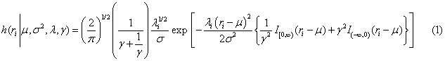
Where the data consists of a single vector of daily index returns, or ri, i =1,…,N. This is an extension of the familiar normal likelihood where in addition to the location and scale parameters as given by μ and σ for the normal case, the parameter vector is supplemented by λ and γ to introduce kurtosis and skewness respectively. These last two unobservable parameters are elicited from the MCMC analysis that estimates the model. In all cases, diffuse priors insure that results are primarily driven by the data.
The FS likelihood function is estimated using MCMC methods because of their unique capabilities. First, MCMC output as a Markov chain providing a large number of parameter values gives a complete description of the parameter. Second, and most important, the Markov chains represent draws from the parameters’ marginal posterior distributions, meaning that parameter values are contingent only on the data. Thus, overall volatility is effectively partitioned among the three components of scale, skewness and kurtosis.
Data augmentation (Tanner and Wong [25]) is used to replicate the Student-t representation of kurtosis by a scale mixture of normals, giving a sampling density of
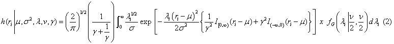
Where, fG is a gamma density specified by degrees of freedom, ν. Thus, each observation ri, i = 1,…., N has a mixing parameter λi, i = 1,…, N as defined by theν hyperparameter. The mixing parameter allows replication of a Student-t distribution having less than thirty degrees of freedom and, hence, accommodates various levels of leptokurtosis or “fat tails”. The γ skewness parameter controls symmetry, allocating probability mass to each side of the distribution’s mode. Values of γ>1.0 produce positive skewness or skewing to the right and γ<1.0 produces negative skewness or skewing to the left. Values of γ and λ equal to unity provide the familiar normal likelihood4
The Bayesian model is defined as

where the joint posterior distribution of the model parameters is proportional to the likelihood function times the parameters’ prior distributions and the right side of the equation is used to formulate the full conditional distribution for each model parameter, defined as that distribution for the parameter conditional on the other model parameters and the data. After repeated iterative re-sampling from the full conditional distribution using MCMC methods, such as Gibbs sampling or the more general Metropolis-Hastings (M-H) algorithm, MCMC output as a long Markov chain comprised of candidate draws for the model parameter converges to the required marginal distribution for that parameter. Sampling-based multidimensional integration has been accomplished to determine the required model parameter’s marginal distribution.
For my analysis the Markov chains are all run for 600,000 iterations with the last 50,000 iterates retained as draws from the required marginal distributions. Of these, every fifth iterate is retained to minimize any potential serial correlation, providing Markov chains of 10,000 iterates each for the subsequent analysis. Such MCMC methods now provide a large sample of independent estimates of each model parameter, cross-sectionally independent across the parameter vector and serially independent within each parameter’s Markov chain. The appendix gives specific details about derivations of the sampling distributions and implementation of the Bayesian MCMC analysis.
A quick review of black-scholes option pricing
A European call option can be priced as today’s expectation of the difference between the terminal underlying asset price ST and the strike price k. For an equity option
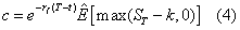
where rf is the risk-free interest rate and T-t is the option’s time to maturity. This is generally represented in terms of the risk-neutral probability of the stock price at maturity, or
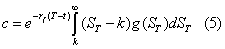
Where, additionally g(ST) is the risk-neutral density of the terminal stock price. The discretized equivalent of equation (5) is
Where S0 is the underlying security’s present stock price and g(ri) is the stock return’s terminal risk-neutral density. The integral in equation (5) is approximated by a summation in equation (6) for very large N representing a large number of small discrete Δri values across a wide range of possible periodic returns. Option prices can now be determined for a wide range of g(ri) specifications. A general g(ri) density can be estimated from historical return data using equation (1) with the mode later adjusted to equate the mean and the risk-free.
Specifically for B/S, the transformation of lognormal discrete returns to their normal continuous-time equivalents by taking the natural logarithm of the price relatives allows the normal specification, N(d1) and N(d2), to be used, or
Where 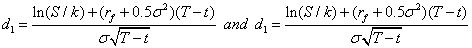
Arnold and Henry [26] derive equation (7) starting with
Where U = ∞ and  . Equation (8) is a specific case of equation (5) for a normal risk-neutral density that, in turn, is equivalent to the continuous-time B/S model of equation (7). Following Brennan [10], in discrete time the mean of the previous lognormal distribution must equal the risk-free rate in order to implement equation (6) using a risk-neutral lognormal density, g(ri). For such a positively skewed risk-neutral specification the mode is not equal to the mean. Hence, the 0.5σ2 (T-t) adjustment is used, giving the mode in equation (8) as
  . In general, pricing call options in a discrete setting using an asymmetric or non-normal risk-neutral density requires first setting the mean of the data-based density equal to the risk-free rate and then finding the resulting mode to realize the new ex post data-based risk-neutral density. This relocation of the databased density to meet the requirement that the mean equals the riskfree rate in order to achieve risk-neutrality is a function of the density’s asymmetry and is termed a “location shift” in this paper. The direction of the location shift is a function of the type of asymmetry or skewness, positive or negative, found for the data-based density. For example, the location shift for the positively skewed lognormal distribution is -0.5σ2 (T-t), a subtraction from the risk-free rate that shifts the distribution to the left and gives the mode shown in equation (8).
Determining the higher moments of the implied risk-neutral distribution
Now that the location parameter for the sought-after implied risk-neutral density has been found, “adjusted” values of the higher moments must be determined from their MCMC data-based marginal posterior distributions. This adjustment that gives “implied” higher moments is accomplished by incorporating call option prices on the S&P 500 index as a proxy for expected market performance5. Jackwerth and Rubinstein [14] discuss incorporation of option market prices into the determination of an implied risk-neutral distribution that produces near model and market price equivalency. Their objective decision criterion is that combination of parameters defining the risk-neutral specification that minimizes the cumulative absolute price difference between proposed model and actual market prices across all strike prices for a call option series of a given maturity. This cumulative absolute deviation (CAD) is defined as
where Ns designates the number of strike prices, i,.…,S, for an option price series of given maturity, Pmodi is the model or intrinsic price from equation (6) for a specific option strike price i and Pmkti is the actual market price of the same option.
As discussed previously each parameter’s marginal posterior distribution given by its respective Markov chain is independent, being contingent only on the data. Thus, candidates to determine new model prices that closely approximate market prices come from independent combinations of the large number of draws comprising each higher moment parameter’s Markov chain. The optimum combination is assumed to lie within the wide range of the parameters’ Markov chains. As such, MCMC output provides a large number of candidate values of each implied higher moment parameter and is a necessary step to then determine specific implied higher moment estimates of the implied risk-neutral distribution. Implementation involves repetitive sampling from all iterates comprising the parameters’ Markov chains. The requirement that the risk-free interest rate is equal to the mean makes a new location shift necessary for each newly proposed risk-neutral specification. The expected value of the CAD is zero, but pricing errors or deviations between implied model and market prices may reflect non-systematic effects or market microstructure noise as discussed by Figlewski [16] that cannot be captured by the parametric risk-neutral specification.
Further thoughts on implied risk-neutrality and implied volatility
Bates [4] and Bing Han [21] show that implied negative skewness results in a volatility “smirk” with increased negative skewness giving a steeper “smirk” and indicating greater bear market sentiment However, this may only address part of the story of implied volatility as a signaling mechanism of future market direction. My simulations (not shown here) indicate that both positive and negative skewness result in volatility “smirks”. IV plots reveal that they lie above the B/S standard deviation regardless of the sign of such skewness. The greater its magnitude, the steeper will be the slope of the resulting IV “smirk”. In both cases, excess kurtosis was present during the simulations.
If familiar IV “smirks” normally occurs, what are the full range of possibilities for the IV plot and the implied risk-neutral density as an information event approaches, especially a major one such as an anticipated equity market “crash”? For example, increased implied risk-neutral market return volatility might be initially expected as market uncertainty increases prior to a major information event. If such uncertainty is later even partially resolved and it does not favor the market, i.e., a bear market looms on the horizon, S&P 500 call option prices should fall, resulting in a decrease in overall implied volatility. IV plot location could change, now lying below a B/S standard deviation based on a previous period of very volatile market return data, as well as IV plot shapes.
Implementation
Model prices are generated for the B/S and ex post risk-neutral distributions per equations (7) and (6) respectively using daily return data for the S&P 500 index for a year prior to an observation date for specific option series maturing during the coming year. Additionally, ex ante model prices for the option series can be generated from their ex post counterparts by the CAD criterion given in equation (9) to determine new model prices more closely approximating actual market prices.
Three series of S&P 500 call options for each of five observation dates in August of 1999, 2002, 2006, 2007 and 2008 are investigated. August, 2008, is chosen as an observation period since it occurs just prior to the steep market decline that began in September as shown in Figure 1 and discussed previously in the introduction. The specific observation date chosen in August was purely arbitrary. The other August observation dates for previous years were chosen to maintain consistency over the time periods of the study. Tables 1-3 give results for the 1999, 2007 and 2008 observation dates6. Each panel of each table representing a call option series of specific maturity gives statistical parameters for three risk-neutral densities; model 1 - the ex post B/S normal density, model 2 - the ex post or data-based nonnormal risk-neutral density, and model 3 - the ex-ante implied riskneutral density . Model 3 incorporates MCMC values for the higher moments that minimize the CAD after sequentially going through all possible combinations of 10,000 sorted draws retained as MCMC output for each of these three parameters7. For each combination of parameter values the mode is adjusted to ensure that the mean equals the risk-free interest rate. The Markov chains are sorted in order to perform Bayesian-based statistical testing of differences between respective ex post and ex ante risk-neutral densities. For example, for the ex post physical specification the median, i.e., iterate 5000 shown in parentheses in the tables, is chosen as the best point estimate of each of the three parameters specifying the three higher moments. The corresponding parameter value for model 3, the ex ante risk-neutral density, also shows an iterate value in parentheses that minimizes the CAD. If such an iterate is less than 250 or greater than 9750 out of a total of 10,000 iterates retained for each of the higher moments’ marginal posterior distributions, then a null hypothesis that the two parameters for models 2 and 3 in that panel are equivalent can be rejected at a 5% significance level. Similarly, a value greater than 9950 or less than 50 is a 1% test and a value greater than 9500 and less than 500 reflects a 10% test. This Bayesian highest posterior density (HPD) estimate for the parameter posterior density is analogous to p-values used for frequentist hypothesis testing. The tests assume that if models 2 and 3 have significantly different parameter values specifying a higher moment at one of the above confidence levels, then the models as given by the corresponding risk-neutral densities are also significantly different. Additionally, the CAD quantity per equation (9) measuring the cumulative absolute price deviation between the given market and each of three model prices is also given in the tables.
| Panel A. December 1999 S&P 500 call options. | ||||
| σ (%) | skewness (γ) | kurtosis (DF) | CAD($) | |
| Model 1: Black-ScholesModel 2: Ex post physical risk-neutral density Model 3: Ex ante implied risk-neutral density+ | 22.2719.56(5000)2* 16.65 (1201) | 1.0 0.94 (5000) 0.56 (1) |
30.0 2.42 (5000)45.24 (8801) |
123.86 162.71 8.29 |
| Panel B. March 2000 S&P 500 call options. | ||||
| σ (%) | skewness (γ) | kurtosis (DF) | CAD($) | |
| Model 1: Black-ScholesModel 2: Ex post physical risk-neutral density Model 3: Ex ante implied risk-neutral density+ | 22.27 19.56 (5000) 17.75(2401) |
1.0 0.94 (5000) 0.56(1) |
30.0 2.42 (5000) 28.61(7601) |
102.99 155.17 2.48 |
| Panel B. March 2000 S&P 500 call options. | ||||
| σ (%) | skewness (γ) | kurtosis (DF) | CAD($) | |
| Model 1: Black-ScholesModel 2: Ex post physical risk-neutral density Model 3: Ex ante implied risk-neutral density+ | 22.27 19.56(5000)15.79(510) |
1.0 0.94(5000) 0.56(1) |
30.0 2.42(5000)7.88(3230) |
92.60 145.82 2.18 |
+ Model 3 is significantly different from the corresponding model 2 specification at either 1%, 5% or 10% significance levels based on the Bayesian highest probability density (HPD) statistic.
* Iterate from sorted Markov chain associated with the parameter value given. For model 2 parameters it is that iterate associated with the median.
Table 1: S&P 500 call option risk-neutral specifications. Ex post risk-neutral density is determined from daily return data for one year preceding the 8/2/1999 observationdate. The ex-ante implied risk-neutral density is derived from the cross-section of strike prices for a specific option maturity using the CAD criterion, i.e., minimizing the sumof the absolute price differences between the model and actual market option prices.
| Panel A. December 1999 S&P 500 call options. | ||||
| σ (%) | skewness (γ) | kurtosis (DF) | CAD($) | |
| Model 1: Black-Scholes Model 2: Ex post physical risk-neutral density Model 3: Ex ante implied risk-neutral density+ |
10.43 7.05 (5000) * 8.69 (9350) |
1.0 0.89 (5000) 0.642 (191) |
30.0 3.79 (5000) 2.43 (2120) |
310.95 411.61 142.29 |
| Panel A. December 1999 S&P 500 call options. | ||||
| σ (%) | skewness (γ) | kurtosis (DF) | CAD($) | |
| Model 1: Black-Scholes Model 2: Ex post physical risk-neutral density Model 3: Ex ante implied risk-neutral density+ |
10.43 7.05 (5000) 8.84 (9580) |
1.0 0.89 (5000) 0.619 (71) |
30.0 3.79 (5000) 2.10 (1320) |
226.82 343.25 27.21 |
| Panel A. December 1999 S&P 500 call options. | ||||
| σ (%) | skewness (γ) | kurtosis (DF) | CAD($) | |
| Model 1: Black-Scholes Model 2: Ex post physical risk-neutral density Model 3: Ex ante implied risk-neutral density+ |
10.43 7.05 (5000) 7.61 (6820) |
1.0 0.89 (5000) 1.21 (9790) |
30.0 3.79 (5000) 2.75 (2920) |
273.47 409.99 74.11 |
+ Model 3 is significantly different from the corresponding model 2 specification at either 1%, 5% or 10% significance levels based on the Bayesian highest probability density (HPD) statistic.
* Iterate from sorted Markov chain associated with the parameter value given. For model 2 parameters it is that iterate associated with the median.
Table 2: S&P 500 call option risk-neutral specifications. Ex post risk-neutral density is determined from daily return data for one year preceding the 8/1/2007 observation date. The ex-ante implied risk-neutral density is derived from the cross-section of strike prices for a specific option maturity using the CAD criterion, i.e., minimizing the sum of the absolute price differences between the model and actual market option prices.
| Panel A. December 1999 S&P 500 call options. | ||||
| σ (%) | skewness (γ) | kurtosis (DF) | CAD($) | |
| Model 1: Black-Scholes Model 2: Ex post physical risk-neutral ensity Model 3: Ex ante implied risk-neutral ensity+ |
20.87 18.86 (5000)* 15.72 (680) |
1.0 0.97 (5000) 0.73 (440) |
30.0 11.92 (5000) 10.33 (4380) |
132.51 160.03 51.00 |
| Panel A. December 1999 S&P 500 call options. | ||||
| σ (%) | skewness (γ) | kurtosis (DF) | CAD($) | |
| Model 1: Black-Scholes Model 2: Ex post physical risk-neutral density Model 3: Ex ante implied risk-neutral density+ |
20.87 18.86 (5000) 15.14 (410) |
1.0 0.97 (5000) 0.79 (1170) |
30.0 11.92 (5000) 10.37 (4400) |
112.19 151.78 40.00 |
| Panel A. December 1999 S&P 500 call options. | ||||
| σ (%) | skewness (γ) | kurtosis (DF) | CAD($) | |
| Model 1: Black-Scholes Model 2: Ex post physical risk-neutral density Model 3: Ex ante implied risk-neutral density+ |
20.87 18.86 (5000) 1.23 (-889) |
1.0 0.97 (5000) 1.05 (7770) |
30.0 11.92 (5000) 1.85 (271) |
1330.98 1418.04 88.57 |
+ Model 3 is significantly different from the corresponding model 2 specification at either 1%, 5% or 10% significance levels based on the Bayesian highest probability density (HPD) statistic. * Iterate from sorted Markov chain associated with the parameter value given. For model 2 parameters it is that iterate associated with the median.
Table 3: S&P 500 call option risk-neutral specifications. Ex post risk-neutral density is determined from daily return data for one year preceding the 8/1/2008 observation date. The ex-ante implied risk-neutral density is derived from the cross-section of strike prices for a specific option maturity using the CAD criterion, i.e., minimizing the sum of the absolute price differences between the model and actual market option prices.
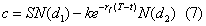
Figures 2-4 supplement Tables 1-3 respectively by showing the models’ 1-3 IV plots. Model 1, designated ‘B/S’, is simply the B/S standard deviation. Model 2 IV’s, designated ‘model’, are based on model prices determined from equation (6) using the ex post riskneutral pdf. Model 3 IV’s, designated ‘market’, use actual market prices that closely approximate prices generated from the ex-ante implied risk neutral pdf’s by using the CAD criterion.

Figure 2: Implied volatility for a sample of S&P 500 call options on the 8/2/1999 observation date. Moneyness is defined as the ratio of strike price to market price. Index level=1328.05.

Figure 3: Implied volatility for a sample of S&P 500 call options on 8/1/2007. Moneyness is defined as the ratio of strike price to market price. Index level=1465.81.

Figure 4: Implied volatility for a sample of S&P 500 call options on 8/1/2008. Moneyness is defined as the ratio of strike price to market price. Index level=1260.31.
Tables 1-3 show the three risk-neutral density specifications for three (1999, 2007 and 2008) of the five observation dates. For all five observation dates eleven of the fifteen option series exhibit model 3 pdf’s that are significantly different than their model 2 counterparts at 1%, 5% or 10% significance levels due to significant changes in scale, kurtosis and/or skewness. Of these, nine are due to significant changes in skewness; eight increases in negative skewness and one increase in positive skewness, three decreases and one increase in scale and one increase in kurtosis. Generally it appears that incorporation of option prices as a proxy for investor sentiment about future market performance produced significantly different implied risk-neutral specifications compared to their data-based ex post counterparts, revealing a bearish outlook relative to the recent past specifically due to increases in negative skewness, but not necessarily indicating increased uncertainty caused by an overall increase in implied risk-neutral volatility. Kurtosis does not play a major role. In all cases model 3 specifications incorporating market prices significantly reduced CAD amounts compared to those of models 1 and 2.
For the 1999 and 2007 observation dates standard deviations for models 2 and 3 are not significantly and systematically different from each other. However, both sets are systematically less than the B/S standard deviations of model 1. This is expected since the B/S normality assumption summarizes non-normal return volatility only by standard deviation which is inflated by the presence of skewness and kurtosis. However, comparison of models 2 and 3 for the March and June, 2009 option series reveals significant increases in negative skewness and decreases in standard deviation with unchanged kurtosis. Such increases in negative skewness indicate a significant increase in investor pessimism about future market performance during the first half of 2009 relative to the earlier 2007-2008 historical period. The reduced standard deviation is the major reason for a decrease in overall implied volatility resulting from low call option market prices. This leads to the conclusion that the bearish market outlook is accompanied by low uncertainty that such will occur.
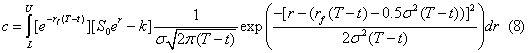
An illustration that this hypothesized decrease in overall return does in fact occur is shown in Figure 5. The difference in return volatility for the implied risk-neutral densities relative to their B/S counterparts is readily seen for the March, 2008 and 2009 option series. For the March, 2008 call options the greater implied volatility seen in panel (a) results from higher market prices relative to B/S model prices. However, in panel (b) the smaller implied risk-neutral return volatility relative to that for B/S for March, 2009 results from reduced market prices relative to those from B/S.

Figure 5: An Illustration of Implied Risk-Neutral Probability Density Functions for Two S&P 500 Call Option Series. The difference in overall dispersion between the implied pdf’s and their respective Black-Scholes counterparts is readily obvious and results in different IV curves.
Radical changes occur for the August, 2009 model 3 implied riskneutral specifications compared to its model 2 counterpart as well as for the previous March and June, 2009 model 3 densities. The August, 2009, option series reveals a model 3 specification having an extreme decrease in standard deviation accompanying an extreme increase in excess kurtosis with a complete absence of skewness. The decrease in standard deviation is so large that it is outside the range of values provided by the data-based Markov chain. The MCMC output iterates are artificially supplemented as indicated by the negative iterate for shown in panel C of Figure 3. We now have a symmetric implied riskneutral density with greatly reduced standard deviation and very “fat” tails. It seems that asymmetric market uncertainty, i.e., “bearishness”, has been replaced by symmetric uncertainty due to the large increase in kurtosis. Simulation evidence indicates that overall risk-neutral volatility increases are limited by increases in kurtosis8. Thus, a large decrease in standard deviation should dominate an accompanying large increase in kurtosis, thus reducing overall implied market volatility. However, the presence of such high levels of leptokurtosis or “thick tails” indicates a relatively higher probability of “extreme” performance, either to the upside or downside. Thus, we might conclude that in August, 2008, reduced long-term call option prices were generally signaling reduced and directionless overall market uncertainty. It seems that long-term investor sentiment revealed a high probability of continued market underperformance accompanied by the possibility of some surprises along the way.
IV plots shown in Figures 2-4 for the 1999, 2007 and 2008 observation dates supplement previously discussed results from Tables 1-3. Model 2 IV plots all exhibit volatility “smiles” or “smirks” and lie above the B/S standard deviation for call options that are in-the-money which later may or may not cross the B/S standard deviation line. As expected, data-based higher moments that exhibit significant skewness and kurtosis have higher model prices than those from B/S in spite of reduced standard deviation. The model 3 IV’s for the 1997 and 2007 observation dates do not present any unexpected surprises, also largely exhibiting IV “smirks” that lie above their corresponding B/S standard deviations.
However, the 2009 call option series exhibit anomalous IV plots lying below their B/S standard deviations. The IV plots also exhibit IV “frowns”, not “smirks”, which largely occur because market prices for the in-the-money call options relatively so much lower compared to those for the other strike prices result in lower implied IV’s. The August, 2009 option series provides the most interesting anomalous IV plots. Here a situation presents itself where such extreme relative market underpricing occurs that the IV’s approach zero, i.e., market prices are so low that B/S equivalent prices cannot be realized, at all strike prices.
Thus, summarizing our findings from Table 3 and Figure 4, by mid-2008 call options of varying maturity were underpriced relative to historical data-based model prices, such as from Black-Scholes, resulting in reduced overall risk-neutral volatility and anomalous implied volatility plots. Though such reduced volatility indicated reduced overall investor uncertainty, high levels of implied negative skewness signaled continuing bearish investor sentiment through the first half of 2009. After mid-2009 high levels of negative skewness disappeared. Thus, by mid-2008 investor sentiment was of increased certainty that the pending market downturn would occur and worsen through the first half of 2009. Longer term S&P 500 index call options maturing after mid-2009 indicated continuing investor certainty that the equity market downturn would persist, but with slightly increased probability that “extreme” market performance could occur, either up or down.
Can option prices give insight into investor expectations, thus providing some indication of future market performance? Using S&P 500 index return data and call option prices to derive the implied riskneutral return distribution, the answer is yes. Utilizing the unique capabilities of Bayesian MCMC empirical methods, results show that investor sentiment clearly signaled the equity market collapse of 2008- 09. Anomalous implied volatility plots exhibiting volatility “frowns”, not the usual volatility “smiles” or “smirks” for equity options, seen just prior to this significant bear market event reinforce additional findings that all three higher moments of the implied risk-neutral density play an important role in revealing investor sentiment about future market performance.
Further research might involve exploration of put option price behavior during such times of financial distress. For example, if call option prices are significantly less than corresponding B/S prices during times of financial distress, then put options should be very expensive. If so, do violations of put-call parity result? Are option markets segmented?
The MCMC Bayesian model is based directly on the Fernandez and Steel [24] or FS formulation and is presented as

Which states that the joint probability of the parameter vector conditional on the data is proportional to the likelihood function h(.) times the prior specifications. The parameter vector θ={μ, σP2P, γ, λB1B,…,λBnB,} has n+5 dimensions and is specified as for each time period’s index return data. The task at hand is to derive the sampling-based marginal posterior distribution for each parameter, including the degrees of freedom hyperparameter, ν, that drives kurtosis. Gibbs sampling is used to determine marginal posterior distributions of parameters when conjugacy of the likelihood and prior distributions exists and an independent or random walk Metropolis- Hastings (MH) step is used when it doesn’t
1. For the location parameter or mode, the likelihood function shown in equation (A2) along with a diffuse or non-informative normal prior is used to specify the parameter’s full conditional distribution. These are of unknown form and an M-H step is used to sample from the required target density. The diffuse prior specification for location is zero with a large variance. A random walk M-H step using a normal candidate-generating density is used to determine the marginal posterior density of each parameter. When skewness is not present and, thus, a symmetric likelihood exists, it is more efficient to use an independent M-H step with a Student-t candidate-generating density. The starting point for the mode, μ (0), is the mean of the return data vector.
2. Considering the variance, σP2P, a gamma prior is used to derive the full conditional distribution, or
Where θB-iB designates all parameters of the parameter vector except σP2P Drawings can be generated for σP2P using Gibbs sampling. The data-based residual variance is used as a starting point when generating the Markov chain.
3. For the kurtosis parameter, λ, a gamma prior is specified, or  , where ν is degrees of freedom. Thus, the full conditional distribution is

and random draws for λ can be made using Gibbs sampling. The conditional distribution for hyperparameter, ν, depends on its prior, which FS specify as an exponential distribution with density,  .This leads to
  where
where  . Thus, we have
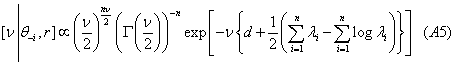
To have a diffuse prior, FS set d = 0.1, thus giving a prior mean of 10 and a prior variance of 100. The above full conditional distribution for ν is not of known form and since >0, a random walk M-H step with a lognormal candidate-generating density is used. Since the degrees of freedom parameter is not observed, a starting value, νP(0), equal to 20 is used. This assumes, a priori, the absence of kurtosis. The subsequent analysis will then show if kurtosis exists.
4. To derive the full conditional distribution for γ, a diffuse prior on ϕ≡γP2P is specified as  . This prior along with the non-normal likelihood gives
As FS point out, this distribution is not of any standard form, but is unimodal. Since φ>0, a random walk M-H step with a lognormal candidate-generating density is used again to draw from the required distribution. Since the skewness parameter is also not observed, a starting value, φP(0), equal to 1.0 is used. This assumes, a priori, the absence of skewness.
The Markov chains are all run for 600,000 iterations with the first 550,000 discarded as the burn-in period. Of the remaining iterates every fifth one is retained to minimize any potential serial correlation, providing Markov chains of 10,000 iterates each for the subsequent analysis. For the M-H steps, all parameters have acceptance rates between 25%-75%, well within the 20%-80% recommended by Bayesian empiricists.
1The symmetric volatility “smile” is more commonly seen for individual securities whereas the asymmetric volatility “smirk” is associated with equity indices.
2Such option price behavior may be interpreted as a violation of put-call parity which says that a more expensive put should be accompanied by a more expensive call. However, there is recent evidence that significant deviations from put-call parity do occur (Cremers and Weinbaum, [5]; Garleanu, Pedersen and Poteshman, 2009; Atilgan, Such price deviations occur due to the trading activity of informed investors as upcoming information events approach.
3I also wish to thank my good friend and colleague, Professor Kenneth Daniels of Virginia Commonwealth University, for providing a portion of the historical option price data used in this paper.
4A λ=1.0 giving zero kurtosis requires degrees of freedom approximately equal to 30.
5Of course, a similar analysis could be conducted for put options on the market proxy.
6Table 1 and its associated Figure 2 for 1999 are also representative of the 2002 and 2006 observation dates. Thus, though the 2002 and 2006 are discussed, their tables and corresponding figures are omitted.
7This implies that the number of potential combinations is on the order of 1012. Implementing various grid search techniques effectively reduced the number of plausible combinations.