Journal of Proteomics & Bioinformatics
Open Access
ISSN: 0974-276X
ISSN: 0974-276X
Research Article - (2023)Volume 16, Issue 1
The current article opens the door for practical implementation of multinomial rejoining tree while citing trinomial rejoining tree as an example where valuation of project increases substantially. When a failure happens at an intermediate stage, based on information and data generated in the process which lead to failure at that stage, as well as based on risk appetite, the project manager or investor can re-invest a fraction of the original planned cost for that stage, to possibly get success. This is how practically problems are being tackled in real world project management, and so it should be for biomedicine. This practical approach is being captured by a new financial mathematical model of trinomial rejoining tree with risk-appetite factor incorporated into it. This method results in much higher valuation than previously known methods, and the method is a more realistic representation of how a manager should take care of finances for a project such as in bioinformatics or software development.
Financial bioinformatics; Calls; Options; Derivatives; Biomedicine; Biotech; Biopharmaceuticals; Financial mathematics; Valuation
Trinomial risk appetite re-joining tree real options valuation
One of the interesting ways to value a project that may have many foreseeable and multistage interdependent outcomes is a real options valuation methodology. The real options valuation not only takes into consideration the time value of an outcome but also optional outcome of an entire project. Simply considering the Net Present Value (NPV) or Net Present Worth (NPW) [1] of a project is not adequate to evaluate true and possible worthiness of a project in hand that takes nearly a decade to complete until commercialization sets in. This paper is a follow up of the conference publication on this model [2]. Although it is very likely that in the couple of years since publication of this paper in international journal, there might be more similar work that could have been produced, the idea of eventual publication of this work to a journal which is open access is to expand the reach to the financial and scientific world.
The options pricing method thus can help in bridging the gap between a business professional and a research professional as in the details of the merits of the procedure can be captured and tapped into, at different stages, for the true worthiness of the project.
It not only benefits product development, but is also needed for the purpose of government regulation and approval, such as the Food and Drug Administration (FDA) in the USA. A vast majority of such biochemical compounds which can possibly be classified as a successful drug get abandoned and never get to reach the intended consumer market.
Matrix of valuation: The aim of this work is to combine the steps from the technical and business perspective starting from the point of data generation to commercialization while using financial instruments of real options valuation to generate a matrix of valuation at different stages. However, even if not purchased, investments at every stage can always be thought of as a call or a put derivative as we would eventually illustrate. The valuation generated is the key component and fundamental step that needs to be done with a lot of precision before getting into the M and A negotiation table.
The valuation of research outcome becomes more critical for independent labs that do not have huge investments backing them up to see outcomes in a span of 5-10 years. These independent labs though based within hospitals or academic clinics well operated by a combination of state/federal government grant money along with short-term support from corporations.
Volatility factor in ‘Big Data’ personalized genomic medicine era
Another factor that would be critical to the successful modeling of an intermediate or final stage of a project would be the associated volatility. Volatility in many ways is a representation of the risk associated of a project to be successful or not. High volatility would imply high risk. Volatility can in many ways be regarded as the standard deviation of a normal distribution. A high standard deviation implies that you are indifferent towards how much people react and penalize or boost the stock price, and that would imply a risk loving behavior. A more sensible way to consider low risk is by keeping lower standard deviation as that would also help in calculating the true optional valuation of the project and such investor are ‘risk averse’.
Predictable product shifts
One reason for reducing the permissible risk is to way-less than one standard deviation, σ, in an intermediate or final stage is due to the fact that with tremendous support from informatics and heuristics systems for knowledge base, such as bioinformatics and pharmacogenomics in the case of pharmaceutical firms, much of the responsibility to device correct and more predictable product shifts in the first R and D phase itself, thereby proposing more promise for a successful implementation of the project in future stages.
Residual factors
Traditional models of valuation even by real options method typically assigned a return value of zero if an intermediate stage is a failure. This can perhaps be revised as even in the worst of case of complete deadlock in moving ahead, there lies some residual value such as cross usage of production components such as software, or the compound to any other project. This residual factor of some value generation even if the milestone of intermediate step was not achieved, as further substantiated by the fact that the company is willing to re-invest a fraction of the original budget for that step, would clearly be more promising news to those who have vested interest in the firm’s activity such as the share market.
The trinomial rejoining tree model proposed in this paper thus also serves to reduce the adverse effect of stock price reaction that the company would have faced if it used the previous binomial tree model such as in article of Shockley, et al. [3].
The challenge thus lies with the management to well understand the non-myopic nature of re-usability of the components, staffs, sub-product of the project in another project, and most importantly, determine the right fallback valuation of the project depending on the stage.
Risk-neutral probabilities
An important concept that needs an understanding is the risk-neutral probability [4,5]. Risk neutral probabilities are the probabilities of future outcomes adjusted for risk, which are then used to compute expected asset values. Once the risk neutral probabilities are calculated, they can be used to price every asset based on its expected payoff [4,5]. A key concept in determining risk neutral probability is to avoid arbitrage possibility. In other words if we for instance have 0 sum at the moment then the probability of going up q multiplied by the reward money of up transition, summed to probability of going down(1-q) multiplied by penalty of going down should be 0.
0=q × Reward+(1-q) × Penalty
However, for sum not starting at 0, the left-hand side of the equation will be that value and the penalty need not be negative. For more than 2 branches of possible outcome, all outcomes are multiplied with their reward/penalty and summed up.
It should be kept in mind that these values are theoretical and real-world probabilities are different. Nevertheless, it gives a good starting point for asset valuation, which the investor can then vary based on his risk appetite of how the prospects can change. The risk-neutral probabilities are applied for binomial, trinomial or multinomial tree in a backward fashion to get the value of intermediary stage and ultimately the first stage of investment, since the return of investment would start from the ultimate branch point where the end consumer pays for the product or where the B2B sales point kicks off or B2P2B where B stands for business and P for platform such as over a software application.
Trinomial re-joining tree valuation model without risk-appetite
Below in Figure 1 for the sake of 2-dimensional figure simplicity, an example of a trinomial rejoining tree is given with the major steps shown. The major steps would be carried out in timely manner as stated if each stage is successful i.e., V25 stage is followed by V22, followed by V17, followed by V10 and lastly V1. Note that the prefix V is used to denote ‘value’ at that stage, and as you must have already noted that projects that does not succeed also have some values in it due to the various reasons stated in my arguments earlier as there are still many points of M and A possibility and complete sale possibility. Not to forget the trained staff in that stage is also an asset at least for the routine operation of not-so-complicated or semi-skilled work that can be put on table for negotiation. A formal calculation of valuation by risk-neutral probability will be discussed later.
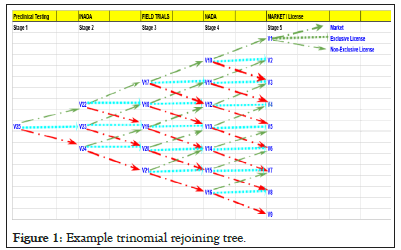
Figure 1: Example trinomial rejoining tree.
Below Table 1 lists some of the key parameters that can be used for different stages using statistics for upward, downward jumps and horizontal movement based previous known recent data for that stage such as time for completion, success and failure rate if the method applied for that stage is already known to be more or less the same as one used by current practice. These parameters are those for trinomial rejoining tree [6,7]. The risk free parameter used is ‘r’ and the discount rate is kept as ‘d’, the values for which can be adjusted as per the greed, desire or market competition for the sector. Transition probabilities are also stated. Theoretically speaking if for example if a project from V25 stage does not succeed to reach V22 successful stage, it can either end up as a near failure such as V24 stage or with possible results of hope but not complete success as desired such as V23.
| Parameters | Values | Constants | |
|---|---|---|---|
| Half sigma | Sigma H=0.5*(sigma) | Risk -Free rate, r | 5% |
| Jumps | - | Discount rate, d | 11% |
| Upward jump size | u=e((Sigma H) *sq.(2*delta T)) | ||
| Movement horizontal | m=1 | ||
| Downward jump size | d=e(-(Sigma H) *sq.(2delta T)) | ||
| Dummy variables | |||
| Dummy 1 | a=e((r*deltaT)/2) | ||
| Dummy 2 | b=e(-Sigma H *sq. root (deltaT)/2)) | ||
| Dummy 3 | c=e(Sigma H) *sq. root (deltaT)/2)) | ||
| Transition probability | |||
| Up | pu=((a-b)/(c-b))2 | ||
| Down | pu=((c-a)/(c-b))2 | ||
| Middle | pu=1-pu-pd | ||
Table 1: Trinomial rejoining tree model parameters.
As delta T varies for every stage and so does sigma, the value of u, d, Pu, Pd and Pm will vary for every stage. A trinomial tree at stage V1 is added and not on other variables because only if the product is successful can one think of going to market on own or going for a license or a combination such as a non-exclusive license. Theoretically speaking, an aggressive investor might not loose complete hope even when the first stage would reach V24 failure stage and might want to invest an amount to get back to success stages. Similarly, a reasonable investor, though despite having option to sell assets and values generated at V23 intermediate success stage might still want to invest time and money to get back to success stage as there are still possibilities as shown by green arrows going upward.
Trinomial re-joining tree valuation model with reinvestment risk-appetite TTHA parameter
Reinvestment fraction: A parameter ‘reinvestment fraction’, ‘ठ’ (pronounced ‘ttha’ from Hindi word derived from Sanskrit) can be used to match the risk appetite of the investor where the Sanskrit word (pronounced ‘tthagna’) implying finding a loophole in the trade tells the merit of the reinvestment process for the investing firm.
Let us say that the investment required for an intermediate stage to go to the success stage such as for stage 2 would be ठ* |V22-V23|. Note that this reinvestment fraction parameter can be applied for any stage, but obviously not the starting stage. Clearly, if ठ is ≥ 1 then there is no sense in the reinvestment process. For cases where ठ is ˂1 then the investment is worth the time. At this stage an evaluation whether to sell the assets or to go for a re-investment is totally dependent on the value of ठ. How actually this reinvestment fraction changes and increases the overall valuation incorporating changes to risk-neutral probability of the project will be discussed in later section of the paper.
A realistic situation can arise when despite one intermediate success stage the company manages to reach V2 stage, but unfortunately missed out the initial plan for time to market and a competitor already got into the market at that stage. So the company would evaluate its option of a ठ*|V1-V2| and would see if it makes sense to quickly get into the market again with the investment and gain market share, or think of negotiating with the competitor for M and A possibilities.
Yet, a further revision of the model would state that the failure of next stage investment will at least retain the value at the previous stage. Here again, assuming not much changes in the market in terms of competition, in terms of value of worthiness of certain milestone already achieved, and the failure of new investment search does not in any way undermine previous achievement. In that case the figure 2 would be a more realistic realization of the value, and we will go by this. Note that in this model the reinvestment of factor ठ has to be done with the next successful stage which is horizontally achieved.

Figure 2: Timeline of R and D stages for Wahoo Genomics investment in a drug for a food animal.
For instance if V4 was the intermediate success result of previous stage of V5, then an investment at V4 can result in success V2 which is greater than V3, the possible success value of previous stage at V5. A semi-success at V4 can result in V3. Speaking in practice, this simply means that an investor just expects a semi-success to be achieved at a stage i.e., a horizontal movement in this model, and for which he would invest if the investment is ठ |V4-V3| where ठ<1. In practice a normal investment would be done if ठ<0.5.
Valuation of project stages by making a case
Now, for the sake of argument to see how the model would fit into the study, we decided to compare the model using the same numbers and events of a similar study that was conducted for a company called Wahoo Genomics Inc. [3]. Below, in Figure 2, you get to see the major steps considered and the proposed investment in each stage.
To briefly explain each step, the Food and Drug Administration (FDA) tightly regulates the approval process through a sub-agency called the Centre for Veterinary Medicine (CVM). In the preclinical stage Wahoo genomics will conduct laboratory testing to see if the drug has any possible promise or not. This again can be a possible success, possible failure or an intermediate horizontal move of hopes, as per our trinomial rejoining tree model, and the investor can decide accordingly based on the risk appetite and reinvestment fraction, ‘ठ, needed to go ahead. Company officials expect this to take 18 months and cost $2 million.
Based on previous historical data, a probability of 5% of its success can be applied. After the completion of preclinical testing phase, Wahoo Genomics will initiate the formal approval process by asking the FDA for Investigational New Animal Drug Application (INADA). This stage can take up to 6 months and can cost $1 million. INADA provides very specific guidelines for how the new drug must be tested as well as for the disposal of the tested animal. The probability of success for this stage by itself is 75% (Figure 3).
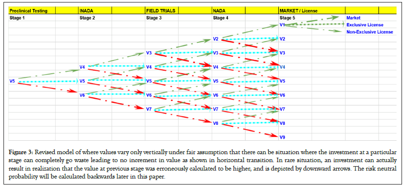
Figure 3: Revised model of where values vary only vertically under fair assumption that there can be situation where the investment at a particular stage can completely go waste leading to no increment in value as shown in horizontal transition. In rare situation, an investment can actually result in realization that the value at previous stage was erroneously calculated to be higher, and is depicted by downward arrows. The risk neutral probability will be calculated backwards later in this paper.
Credibility of data: On grant of INADA, field trials can begin which typically can take 2 years and would could about $5 million as per previous data estimation.
This stage in itself has been reported to have a success rate of about 25%. The next stage would be the New Animal Drug Application (NADA) to the FDA. This stage would cost $ 0.5 million and has a 75% possibility of success at this stage. Even after approval or before that the company can look at the competitor behavior and market changes and respond accordingly since there will be investment of the order of $10 million to channel the drug to end customers. Other options to consider would be granting non-exclusive license to another firm or go for subsidiary channel and explore other M and A options that would best suit the status of market competition at that moment. The total probability of success going through all the stages would be 0.0 × 0.75 × 0.25 × 0.75=0.007 or 1 in 142 (Figure 4).
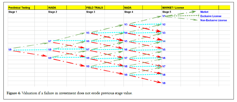
Figure 4: Valuation if a failure in investment does not erode previous stage value.
For sake of simplicity based on historical figures as reported in article [3], the initial penetration rate of 3% can be considered, and given that the drug is successful, the penetration rate can increase up to 50% over 10 years, and this can be used for accumulating the wealth generated, that can be discounted back to current year, assuming a very conservative market size of only $85 million per year.
After 10 years, there will be substitutes and competing products that would be launched and would lead to negative penetration and thus declining market size to be considered for revenue. Please also note that we are currently in 2002 as that is when we would be able to make a fair comparison with the binary model proposed by at that time to the revised trinomial rejoining tree model as discussed in this paper, and for comparison sake, the numbers and assumptions have also been kept the same as that used earlier. It should be emphasized that the model can work pretty much in good form for current year of 2017 or beyond. Table 2 below gives some of the assumptions used for various calculations needed later.
| Assumptions per year | Discounted (%) |
|---|---|
| Expected market size per year | $85 million |
| Real growth in market per year | 0% |
| 2007 penetration rate | 3% |
| Terminal penetration rate (2017) | 50% |
| Growth in penetration rate | Straight line |
| Cost of goods sold | 30% of sales |
| SG and A expenses | 25% of sales |
| Working capital commitment | 10% of sales |
| Marginal tax rate | 12.10% |
| Cost of launch in 2007 | $10 million |
| Depreciation of launch costs | Straight line |
| Terminal growth rate after 2017 | -20% |
| Real-$ discount rate | 11% |
Table 2: Assumptions as used in article (Shockley, 2002) for Static Discounted Cash Flow (DCF).
Using these values the return on sales for the next 10 years are conditional success of the product approval from all the stages are shown in Table 3 below. Note that the terminal value is accounting for whatever revenue generated for the rest of the years following the 10 year period, given that there is a negative growth rate as discussed earlier.
| Products | Apr-07 | Apr-08 | Apr-09 | Apr-10 | Apr-11 | Apr-12 | Apr-13 | Apr-14 | Apr-15 | Apr-16 | Apr-17 |
|---|---|---|---|---|---|---|---|---|---|---|---|
| Market size | $85 | $85 | $85 | $85 | $85 | $85 | $85 | $85 | $851 | $85 | |
| Market penetration rate | 3.0% | 8.2% | 13.4% | 18.7% | 23.9% | 29.1% | 34.3% | 39.6% | 44.8% | 50% | |
| Sales revenue | $2.55 | $6.99 | $11.43 | $15.87 | $20.31 | $24.74 | $29 .18 | $33.62 | $38.06 | $42.50 | |
| COGS | 0.77 | 2 .10 | 3.43 | 4.76 | 6.09 | 7.42 | 8.76 | 10.09 | 11.42 | 12.75 | |
| SG and A | o.64 | 1.75 | 2.86 | 3.97 | 5.08 | 6.19 | 7.30 | 8.41 | 9.52 | 10.63 | |
| Depreciation | 1.00 | 1.00 | 1.00 | 1.00 | 1.00 | 1.00 | 1.00 | 1.00 | 1.00 | 1.00 | |
| Pretax profit | 0.15 | 2 .15 | 4.14 | 6.14 | 8.14 | 10.14 | 12.13 | 14.13 | 16.13 | 18.13 | |
| Taxes | 0.02 | 0.26 | 0.50 | 0.74 | 0.98 | 1.23 | 1.47 | 1.71 | 1.95 | 2.19 | |
| NOPAT | 0.13 | 1.89 | 3.64 | 5.40 | 7.15 | 8.91 | 10.66 | 12.42 | 14.18 | 15.93 | |
| Add back depreciation | 1.00 | 1.00 | 1.00 | 1.00 | 1.00 | 1.00 | 1.00 | 1.00 | 1.00 | 1.00 | |
| FCF from operations | 1.13 | 2 .89 | 4.64 | 6.40 | 8.15 | 9.91 | 11.66 | 13.24 | 15.18 | 16.93 | |
| Change in NWC | 0.26 | 0.44 | 0.70 | 0.89 | 1.14 | 1.33 | 1.59 | 1.78 | 2.03 | 2.22 | |
| 0.87 | 2 .44 | 3.94 | 5.51 | 7.01 | 8.58 | 10.08 | 11.64 | 13.15 | 14.71 | ||
| Tenminal value | 37.97 | ||||||||||
| Free cash flow | 0.87 | 2 .44 | 3.94 | 5.51 | 7.01 | 8.58 | 10.08 | 11.64 | 13.15 | 52.68 | |
| April 2007 value | $51.63 | ||||||||||
| Cost of launch | $10.00 | ||||||||||
| April 2007 NPV | $41.63 |
Table 3: Sales and revenues for Wahoo Genomics conditional upon product launch as used in article Shockley, 2002.
This Net Present Value (NPV) of $41.63 million need to be discounted back to 2002 year and also probability adjusted for its success by standard DCF model such as shown in Table 4 and when doing so, the valuation would come out to be-$2.02 million which would lead to Wahoo Genomics to stop thinking of even starting this venture.
| Stage | Conditional probability of success in prior stage |
Cu1nulative probability of entering stage | FCF ($ millions) |
Probability weighted FCF ($millions) |
Date | Apr-02 PV using 11% ($ millions) |
|
|---|---|---|---|---|---|---|---|
| Exploratory | Already Completed | ||||||
| Preclinical | 1 | -$2.00 | -$2.00 | Apr-02 | -$2.00 | ||
| Inada | 0.05 | 0.05 | -$1.00 | -$0.05 | Oct-03 | -$0.04 | |
| Field testing | 0.75 | 0.0375 | -$5.00 | -$0.19 | Apr-04 | -$0.15 | |
| Nada | 0.25 | 0.009375 | -$0.50 | $0.00 | Apr-06 | $0.00 | |
| Launch | 0.75 | 0.00703125 | $41.63 | $0.29 | Apr-07 | $0.17 | |
| Apr-02 NPV | -$2.02 | ||||||
Table 4: DCF and probability adjusted NPV.
Need for a more realistic value capture financial valuation model
The NPV analysis done in the previous section would clearly put the investors on back-foot and not proceed further to venture into the business plan. Thus, this would not be a sensible approach for the company needs for a more sensible financial mathematical model.
Financial options of execution: The standard NPV approach is thus misleading as it does not capture the true value of the intermediate and thus overall product especially if there is optionality that this intermediate value can be put into. Summing up different stages, the project will be not just ‘options-on-options’ but ‘Multiple-Options-On-Multiple-Options’ (MMOs). The options-on-options feature is derived simply due to the fact that an option executed at one stage has thus an effect on option that is executed on previous or subsequent stage. Here, as we are in a trinomial re-joining tree, at every stage there is more than one option, and thus multiple option scenarios comes into picture. Clearly, the value of ठ will make an impact in the decision making.
To see this, look forward in time and suppose that the R and D program has been completed through the field trial stage and thus has a value of V5. Figure 5 below shows a realistic decision option a manager is stuck at field trial stage to exercise.
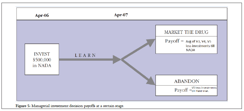
Figure 5: Managerial investment decision payoffs at a certain stage.
As shown in figure 5, an investment manager can expect from investing in NADA stage would be the average of all three possibilities of success V3, failure value which will be the same as in previous stage V5, and semi-success V4, and then deduct the investment required to make a decision.
Figure 6 below represents a European call option scenario where the company can buy the option at the completion of field trial stage by investing $500,000 if the value of the project i.e. average of V3, V4, V5 is greater than $500,000. If not then the company would not invest in call option and simply retrieve value V5.
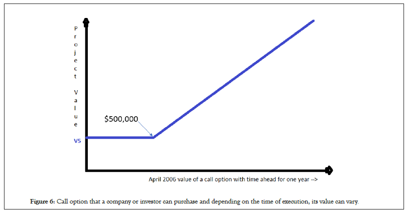
Figure 6: Call option that a company or investor can purchase and depending on the time of execution, its value can vary.
Now stock price in itself cannot be affected by just a single project for a firm unless it's very crucial project. The stock price movement will depend on lot many factors as it is to do with a normal stock price movement as observed in other sectors. Nevertheless, if the project is very critical, or if the project is that of a newly formed public limited company, the stock prices can well be designed and priced as derivatives using the methods and analysis suggested here for valuation of a stage.
Call option parameter
If the project is semi-successful then the next time period zone is achieved where the current value would still be V4 and the value of ठ will come into picture i.e. ठ |V4-V3| can be the call option parameter instead of taking the average of possible outcomes. Once again, if ठ>0.5 (say for a moderate risk taking investor), then clearly the call option can be abandoned, and if ठ<0.5, the option can be exercised. The ठ parameter multiplied by value difference from the closest success would be a better and finer way of call option valuing rather than taking the average of all possible outcomes.
In the field trial stage itself, i.e., at value V5, the investor can decide to invest or not depending on whether $ ठ*|V4-V5|> $500,000 for instance of investment. ठ is in a way calculating the reciprocal of return worthiness of an investment. In this case for instance, $500,000/$|V4-V5| gives value of ठ as >1 if |V4-V5|=$500,000, which implies that enterprise is worth the same risk of return as investment. A moderate risk appetite investor would look for a value of ठ as 0.5 as then its reciprocal is about 2 times the return in investment. In this case if $500,000/$|V4-V5| is greater than 0.5, then for a moderately risk-taking investor, that would be a risky investment, if less than 0.5 it would be an investment worth considering. In any case almost any manager or investor would not mind keeping ठ as 0.1 if there can be possibility of reasonable success within a permissible time-span if that can increase the worth of that stage justifying the sunk cost to be not really a sunk cost, as we discussed earlier.
What value of ठ that matters to an investor is totally personality and project dependent, however, introducing this factor does make a lot of sense to reflect practical and realistic situations (Figure 7).
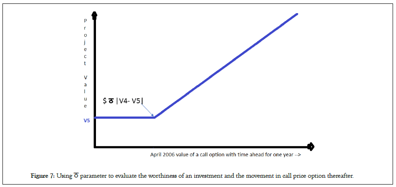
Figure 7: Using ठ parameter to evaluate the worthiness of an investment and the movement in call price option thereafter.
Multiple-options-on-multiple-options explained in detail
MMOs holds good for overall valuation in such valuation techniques where the outcome at every stage is more than two, such as the trinomial re-joining tree model discussed in our case. This is nothing but a chain of options, i.e. options on options, but given that on every option outcome, there can be more than one options applied on it and so it’s named as multiple options on multiple options, instead of just chain of options. It should be noted the MMOs can also hold good if for some reason the branches at any intermediate stage for some reason can be more than 3 as well such as 4 or 5.
Call option pricing
In our trinomial rejoining tree model, as at each step the option can be considered to be having a call price movement of either the average of three possible outcomes or through the ठ way of valuation for the next incremental success possibility. For most calculations ahead the ठ way is chosen for call options pricing at a stage that builds upon option of other stage in similar way. Nevertheless, every stage has three options of investment to pursue and purchase a call option, and that is dependent on how that stage was reached. Was that stage achieved as a result of success from previous stage? If yes, then the investor would likely be interested in purchasing an option call for the next success stage.
The second circumstance could be that if this stage was achieved by horizontal movement say from V5 to V4 and we are currently at V4 and the investor thus does not look too much convinced to invest $10 million to enter V2 stage but would rather invest ठ times the difference of V3 and V4, to see partial success of getting to V3 stage rather than risking to see V2 stage. Yet, at this same situation the investor can also abandon any call option purchase as well. Thus the multiplicity of options by which the option pricing can be set at the stage and builds upon future stages in similar way makes MMOs a much versatile derivative models for trinomial rejoining trees projects.
Building one option on another
Multiplicity of call options also arises due to the basic nature of the problem of multi-stage project itself, since investing at any stage is the same as betting for a favorable return at a future date, but the favorable return at that future date is itself dependent on investing at that stage, which is the same as buying a call option to bet a favorable return at a future date when that stage finishes, and so on and on, thereby essentially building one option on top of another. Figure 8 below lists the various ways by which MMOs build upon for our case.
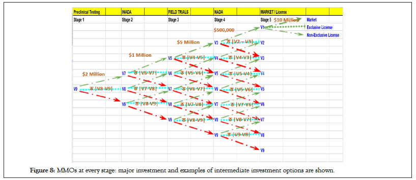
Figure 8: MMOs at every stage: major investment and examples of intermediate investment options are shown.
For sake of simplicity, and clarity of picture not all investment call options are shown. For example an investment of $5 Million will be needed for every points connecting V5 to V3. Similarly, V6 to V4 would need investment of ठ |V4-V6|.
Derivation of financial valuation of MMOs
The underlying assets of all the stages are multiple options with the exception of the last stage for which the estimated cash flow is $51.6 million after entering the market with investment of $10 million at V1 stage. At this stage it can be assumed that if there is no intermediate stage or if they have been already successfully completed then the company can go to market with an option of $10 million. Given what was known in 2002, the expected cash flow in 2007 ‘Present Value’ (PV) was $51.6 Million as stated before. However, we would like to know its current value in April 2002 and not its exercise value in April 2007. Thus applying a discount rate of 11% risk adjusted percentage for DCF analysis, the starting value of the underlying asset is $51.6/(1+0.11)5=$29.8 million.
Volatility
In an option, the volatility of the underlying asset is a measure of how much the underlying asset’s value can change (per unit time) between the initiation of the option and the expiration. In our current context of real options, the volatility can be considered as the uncertainty about the initial estimate of the value of the underlying asset at various stages.
For the time being we can consider volatility (Sigma, σ) of 100% i.e., the true value can be double the amount estimated to almost 0. This volatility figure can be matched to management’s subjective probability of success, as this volatility estimate is a reflection of the risk that the project has to eventually get successful. A low risk project as the management would know would have high probability of success, and since it would hold the same for competitors in market, the return would not be that high. For a high volatility project, which has little chances of getting through the last stage, the risk is very high say more than 300% and so the return could also be very high. Typically, in biopharmaceutical and biotechnology sector, it does not makes sense to keep the volatility risk of less than 100% given the complex uncertainty involved in intermediate stages.
For the sake of simplicity of calculation, apart from volatility factor of 100% per year, each time step taken is of 1/2 a year in the analysis, such that at any step, the next step will have an upward, downward and horizontal jump factor of 1.65, 0.61 and 1 respectively, as we get the values by feeding into the parameters as in table 1. Now realistically, as we stated, a horizontal jump would not be of the order of 1 but a factor of slightly more than 1 since there will be some added value in any case. A realistic add-on could be at least equivalent or proportional to the reinvestment percentage for that stage, i.e., reinvestment risk appetite parameter TTHA, ठ, say 10%, of the difference from upward jump which would be in our case 10% of (1.65-1)=0.065. Thus, the horizontal jump should be adjusted to 1+0.065=1.065. Thus, we would first make a trinomial re-joining tree with keeping horizontal jump value as 1, and then adjust the horizontal values by the effect of ठ. The probability of success, failure and intermediate success after every 6 months would be 0.21, 0.29 and 0.50 respectively for same values of volatility of 100% per year and taking risk free rate of 5% as a modest figure and plugged into the table 1 formulae. Clearly, even under these modest assumptions a very high probability of 50% exists for the project to advance only at horizontal pace of intermediate success. Figure 9 below lists the trinomial tree with re-joining capability without adjustment to horizontal ठ values and with all possible redundancy in values to show how rejoining takes place.
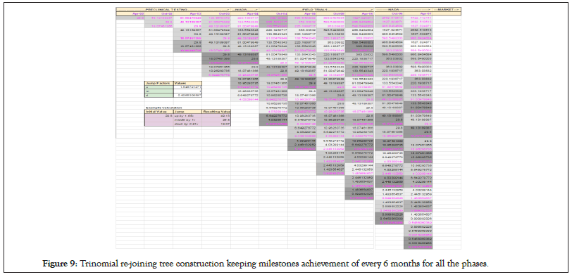
Figure 9: Trinomial re-joining tree construction keeping milestones achievement of every 6 months for all the phases.
The colored values are the unique values which can represent nodes in trinomial tree where multiple branches merge. Figure 9 below shows the valuation at each intermediate stage with only the unique branch node points values displayed (Figure 10).
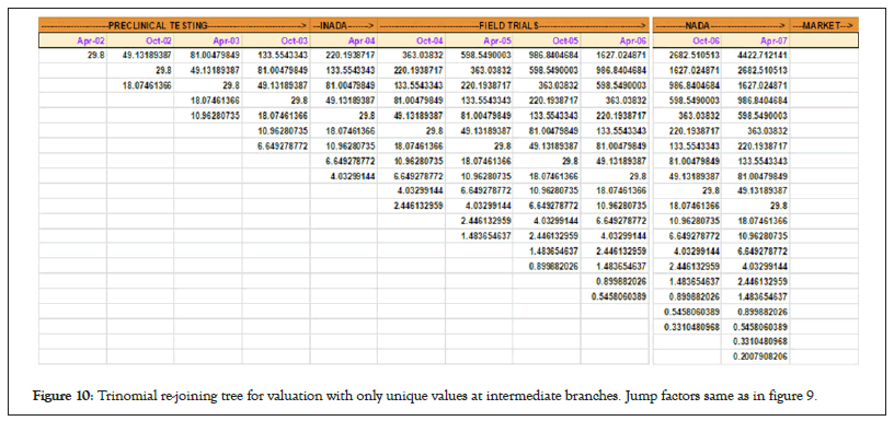
Figure 10: Trinomial re-joining tree for valuation with only unique values at intermediate branches. Jump factors same as in figure 9.
Finally we adjust the values such that the value of reinvestment appetite, TTHA, ठ, is kept to be a reasonable number of growth and progress expected per step of modest 10%. This value can be adjusted as per the risk appetite of the investor for the additional investments he seeks to do for an intermediate result movement. The reinvestment amount that needed due to ठ would be considered at later section for discounting from the overall profit. Figure 11 summarizes the final table of valuation.
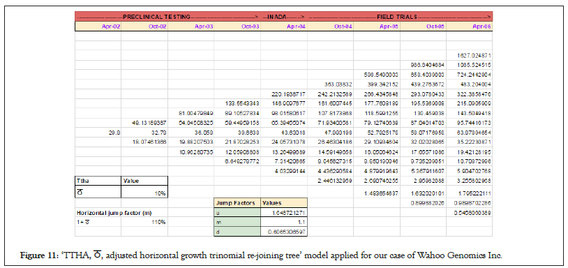
Figure 11: ‘TTHA, ठ, adjusted horizontal growth trinomial re-joining tree’ model applied for our case of Wahoo Genomics Inc.
Next, once we have determined the possible outcomes of revenue at the pre-market state, we can work backward given the profitability situation or business sense of a) exercising a call option of $10 million if it made business sense, or b) simply not exercising the option and so getting a return of zero. This will change the values as in Figure 12 (note that revenues are shown at this stage of discussion and profits will be shown later).The profit would be subtracting 10 Million from the positive numbers which show revenues for those cases where the call was exercised. ‘0’s are for those cases where the call was not exercised.
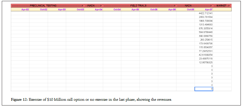
Figure 12: Exercise of $10 Million call option or no exercise in the last phase, showing the revenues.
The cost of purchasing call option before-hand can be always to some extent of more-or-less offset by the intrinsic value generated till that stage where the values are thus shown to be zero. This is because, in reality, the return in ‘no exercise of call option’ cases should not be zero but negative, owing to the fact that there are costs involved in purchase of patent but that can be always covered up by the fact that there are some asset always for sale even in case the project is a failure as you would notice some values in Figure 11 last column which has been put as zero in Figure 12.
We can then work backwards in time by calculating at each trinomial node in October 2006, the expected present value using risk-neutral probabilities and a risk-free discount rate. The latter correctly adjusts for the market risk of the project, which for a risk free rate of 5% and time steps of 6 months is expr × t=e0.05 × 0.5=1.025. The Risk-Neutral probabilities are largely the transition probabilities as was shown in table 1 whose values can be as shown in Table 5 below for the dependent parameter values considered in our case for Wahoo Genomics. The sum of these risk-neutral transition probabilities is always 1.
| Parameters | Formula | Values | Constants | |
|---|---|---|---|---|
| Half sigma | Sigma H=0.5 × (sigma) | 0.5 | Risk-Free rate, r | 5% |
| Jumps | Discount rate, d | 11% | ||
| Upward jump size | u=e((Sigma H) *sq.(2*delta T)) | 1.6487213 | ||
| Movement horizontal | m=1 | 1 | ||
| Downward jump size | d=e(-(Sigma H) × sq.(2delta T)) | 0.6065307 | ||
| Dummy variables | ||||
| Dummy 1 | a=e((r*deltaT)/2) | 1.0125785 | ||
| Dummy 2 | b=e(-Sigma H × sq. root (deltaT)/2)) | 0.7788008 | ||
| Dummy 3 | c=e(Sigma H) × sq. root (deltaT)/2)) | 1.2840254 | ||
| Transition probability | ||||
| Up | pu=((a-b)/(c-b))2 | 0.21411 | ||
| Down | pu=((c-a)/(c-b))2 | 0.2886695 | ||
| Middle | pu=1-pu-pd | 0.4972204 | ||
Note: As deltaT varies for every stage and so does sigma, the value of u, d, Pu, Pd and Pm will vary for every stage. A trinomialtree at stage V1 is added and not orn other variables because only if tile product is successful can one think of going to market on own or going for a license or a combination such as a non-exclusive license.
Table 5: Calculation of transition probabilities which also serve as risk neutral probabilities.
Thus, any node would have a value that is the projection of transition probability weighted value of the 3 nodes that can emerge from it and then discounted back by a factor of risk free discount rate.
Value of a trinomial node={(upward-transition probability) × value of upward resulting node+(horizontal-transition probability) × value of middle resulting node+(downward-transition probability) × value of downward resulting node}/exponential(risk-free rate × time for sub-stage)
Vnode={Pu × Vu+Pm × Vm+Pd × Vd}/ert
Doing it as an example for the first top-most node in October 2006 it will be:
={0.2141100292 × (4422.712141)+0.4972204404 × (2950.761564)+0.2886695304 × (1968.700094)}/1.025=2909.687533 Million USD
If we simply consider the fact that there were no investments needed in intermediate stages, then complete backward calculations using the formula stated above, would look like that in Figure 13.
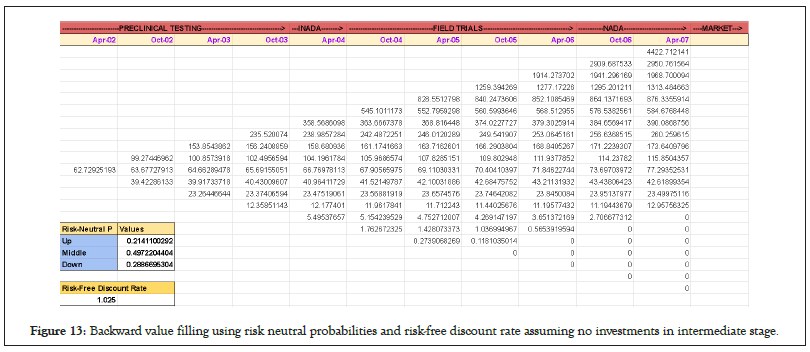
Figure 13: Backward value filling using risk neutral probabilities and risk-free discount rate assuming no investments in intermediate stage.
However, as we know that at each intermediate stage there is an investment needed that can be thought of or actually implemented as a call option and thus if the valuation at that stage is not profitable, the option is not exercised.
This has to be done for every stage and the investment needs to be further processed at each stage showing effective profit instead of pure revenue. For the first stage the graph will look as in Figure 12 with a minor change of deduction of 10 million USD has been either exercised where it made sense or not exercised keeping profit to be 0.
Value generation versus option selection
The same situation can arise in NADA stage in April 2006 where the concern is that does buy the call option of $500,000 in the form of investment (or actually an option) makes sense as the benefits of buying this option would be reaped only a year later in April 2007. However, since their possible valuation given the stage at which the project is, can be evaluated using the risk-free discount rate and trinomial node re-joining methods of risk-neutral probabilities, one can then decide to either a) buy the option or invest and get the profit as valuation at that stage less option price or b) do not exercise option and thus have zero.
The argument that the real value would still not be zero in case 2 still applies as was discussed several times and in previous cases. These two scenarios of call option by first valuation generation and then deciding to go for option or not can be applied at each stage subtracting the investment for that stage such as $5 Million in April 2004 at the field trial stage, $1 Million in October 2003 before INADA stage and $2 Million in before April 2002 to get into preclinical testing phase. The whole chart is shown in Figure 14.
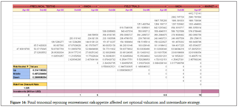
Figure 14: Final trinomial rejoining reinvestment risk-appetite affected net optional valuation and intermediate strategy.
It is important to note that since we are keeping a trinomial re-joining tree as a model, thus the risk-neutral probabilities remain the same in this model, and the real case scenario will be slightly different, as this model serves as a template form for project stage valuation and helping to guide whether to invest or not at a stage as a decision tree.
Subtracting the value of re-investments using TTHA, ठ, factor
A practical application of the model would also involve subtracting the re-investment money needed to go from a complete failure to an intermediate success stage that would be ठ or 10% of the amount for that stage. For steps more than 6 months, the step’s investment can be broken down into sub-steps of 6 months each to get a rough understanding of investment at each stage and thus the value of ठ.
For instance the field trial stage can be broken into 4 sub-stages, thus having a sub-investment of $5 Million/4=$1.25 Million and thus the value of ठ will be 10% of $1.25 Million=$0.125 Million. In reality, only few of the sub-stages might need the addition of ठ, but for argument sake we can take into account the worst case scenario of all the sub-stage of every stage required reinvestment of ठ.
As the final launch to market stage is not considered as a sub-stage, we would not consider that investment to be as part of reinvestment ठ requirement. In that case for the worst-case scenario, the reinvestment amount would be 10% of (2+1+5+0.5) Million USD=10% of 8.5 Million USD=$0.85 Million.
At this time when the final model has been generated, it should be emphasized that there were certain assumptions like volatility of market and penetration in market that were assumed to be a fixed and constant values, can be actually played with in real world scenario.
Real life biotech project examples to demonstrate reinvestment benefits
Example by Drug Reposition Research Work: The outcome of a process at any stage may not be a definitive Success or Failure. Articles [8-10] talk about recent methods using big data from healthcare for the methodology and benefits of drug repurposing. For instance if a project for big data analytics for drug repositioning is done such as [8-10] for one year budget of 100K USD, and in the end of the year there is no successful final result, as per previous models, it will regard 100K USD as a sunk cost.
It will be assumed that the employee's contract is over and that his codes cannot be read by the new employee who joins and thus the money is purely wasted. The current work in this article provides a model that, if after having spent 1 year of time and 100K USD, if there are possible evidences that the results can be achieved if the same staff programmer employee is made to re-check his codes, then it is perhaps more sensible to invest a fraction of that money, say that fraction is ‘TTHA’, ठ, into next stage and that would make the so called sunk cost as non-sunk [11].
Thus, effectively by having spent say just 10 K USD more in re-investment stage on the project instead of initially having estimated 100K as that stage budget, the effective new sunk cost is only 10K instead of whole 100K USD. Clearly, while a traditional means of valuation can lead to lesser valuation, the TTHA affected reinvestment mechanism will lead to a higher valuation. The calculation is not show here, as the calculation was already shown for the Wahoo Genomics case study that was discussed the project might continue by following traditional routes to solve certain biomedical problem or the process in itself might become semi-innovative, resulting in byproduct of additional value other than the initial plan to solve a problem and thus an enhancement in valuation as the by-product opens up new market to explore the enterprise of apart from reputational value in general generated from publication and the grant money from state and federal government that it would likely attract [12-14].
Thus clearly, the values as we see if the board members cleverly and realistically plan and monitor the steps involved can extract out more valuation at each step from the project. The board can also think of selling the intermediate step deliverables to non-competing market to gain additional capital in between if it thinks that by waiting too much can perhaps destroy the value of the product generated in intermediate step, especially if it sees this route as a means to financing its future steps in project and there is a red-ocean competition around.
The net present valuation applied directly by discount rate application gave a value of-$2 Million and the binomial option method of management and thus the valuation as discussed in the article of Shockley, 2002, for the same figures and case study gave a valuation of $19.8 Million. The current model as proposed in this work significantly enhances the management perspective of the project and the valuation associated with it having a tremendous impact on M and A activities at the beginning or at any intermediate stage. The net valuation using this model for same case study and metrics came out to be 2.5 × higher having a significant impact at a figure of $47.91 Million. After discounting the value of re-investment at intermediate stage under worst case scenario as discussed above considering ठ effect, it would be ($47.91-$0.85) Million=$47.06 Million, which is still about 2.5 × higher. The method proposed in article, using just a binary multi-stage call option model, also stated that there was an upper bound of $29.8 million that the project can be valued at no matter how much the volatility figure is adjusted. The current model as is proposed in this article clearly much surpasses the upper-bound that would have restricted the investors to value a project and opens door for valuing project at a more sensible way.
It must also be noted that even though we have used trinomial tree right from the root i.e, beginning of the project, in reality, the beginning of the project 1st phase should have only a binomial tree resulting in either success or failure, and the trinomial tree of reinvestment factor will start from that point onwards where the effect of failure and reinvestment to save the sunk cost gets started.
The value of the risk-appetite parameter, TTHA, can be varied across the Excel sheet formula (provided as supplementary) material, to see where the maxima and minima lies and what optimum value such as the highest practical valuation can be achieved. This work can be also plotted as future work or a mathematical function for valuation which is dependent on TTHA that can be differentiated by calculus methods can also be worked upon to find the optima.
The author was benefited by interactions with Prof Sonja Prohaska at Department of Computer Science and Interdisciplinary center of Bioinformatics, University of Leipzig, for her opinions on biotech sector R and D projects. Ms Saswati Sanyal contributed in formatting the manuscript in APA style.
None to be declared
The calculations were done on Excel sheets which can be downloaded from here: www.tinyurl.com/abinarain and then click on ‘Educational Stuffs’.
[Crossref] [Google Scholar] [PubMed]
[Crossref] [Google Scholar] [PubMed]
[Crossref] [Google Scholar] [PubMed]
[Crossref] [Google Scholar] [PubMed]
Citation: Singh AN (2023) Trinomial Risk Appetite Re-Joining Tree Real Options Valuation: Examples in Financial Bioinformatics. J Proteomics Bioinform.16:629.
Received: 29-Jan-2023, Manuscript No. JPB-23-21602; Editor assigned: 31-Jan-2023, Pre QC No. JPB-23-21602 (PQ); Reviewed: 15-Feb-2023, QC No. JPB-23-21602; Revised: 23-Feb-2023, Manuscript No. JPB-23-21602 (R); Published: 01-Mar-2023 , DOI: 10.35248/0974-276X.23.16.629
Copyright: © 2023 Singh AN. This is an open-access article distributed under the terms of the Creative Commons Attribution License, which permits unrestricted use, distribution, and reproduction in any medium, provided the original author and source are credited.