Journal of Pollution Effects & Control
Open Access
ISSN: 2375-4397
ISSN: 2375-4397
Research Article - (2017) Volume 5, Issue 2
Tropospheric ozone climatology in eastern Equatorial Africa has been at the core of this study. Seasonal and annual tropospheric ozone distribution and variation have been investigated using SHADOZ network data from Nairobi for the period 1998-2013. Meteorological parameters including air temperature, relative humidity, atmospheric pressure as well as ozone partial pressure have permitted to provide the first comprehensible tropospheric ozone climatology over this region. Mean seasonal tropospheric ozone distribution displays two distinct peaks occurring in winter with 43 DU (July) and 46.8 DU in spring (October). Comparison of mean seasonal ozone partial pressure with relative humidity profiles shows a logarithmic trend with strong regression coefficient for ozone partial pressure (0.81
Keywords: Climate change; climatology; impact; model; tropospheric ozone
Tropical and subtropical Africa is considered to be leading sources of air pollution from biomass burning [1]. Although biomass burning is highly rated as the main tropospheric ozone contributing sources in these regions, a few studies on this topic have been undertaken, especially in eastern and equatorial Africa where the levels of tropospheric ozone have been increasing since the last past decades of the 20th century [2]. Tropospheric ozone, as secondary pollutant and a greenhouse gas, has negative effects on human health and the environment. Its concentrations depend on precursor emission levels from natural and anthropogenic activities. Dynamical factors that determine its dispersion and transport into the troposphere also play a crucial role. In recent years, trends on tropospheric ozone have been exacerbated by change on climate parameters at global level. However, in Africa these trends have been poorly documented and understood. African continent, particularly the East Africa, is among the most vulnerable to climate change impacts due to its geographical position and the lack of resilience capacity to mitigate these impacts [3]. This is because observations on ozone concentration over tropical Africa were only available from TOMS (Total Ozone Mapping Spectrometer) instrument aboard the Nimbus 7 satellite and no in situ measurement data existed [4,5].
Previous results from TOMS satellite data in this region displayed elevated ozone levels, which coincided with biomass burning season over the tropics [6-9]. Furthermore, sporadic ozonesonde operations undertaken in the region [10] presented significant uncertainties [4,11], and limited ozone research in the tropics [10,12,13]. Likewise, the lack of ozone profile measurements restricted the assessment of its regional budget, and validation of both global models, and satellite information [14].
In eastern equatorial Africa, Nairobi (Kenya) constitutes the unique site location for the detection of ozone, where a few ozone monitoring campaigns have been undertaken, under the active involvement of the World Meteorological Organization (WMO) through Global Ozone Observing System (GO3OS) [15]. This campaign encompassed monitoring ozone concentrations at the surface using TEI 49C instrument, and the vertical profile, and total column ozone in the atmosphere, using Dobson spectrophotometer number 18, since the year 2005. Monitoring campaign results showed that data from this programme were not consistent until the year 2002, and could not be used for research purpose. Hence, tropospheric ozone characteristics were only studied at individual scale, with no specific characteristics from regional pattern.
Ozone known as greenhouse gas plays negative role in human health [16], on vegetation [17] and in the environment [18,19]. Due to lack of sufficient data in African continent, additional ozone measurement stations distributed in the tropical and subtropical southern hemisphere were launched by NASA’s Goddard Space Flight Center, NOAA/ CMDL (Climate Monitoring and Diagnostics Lab) under SHADOZ (Southern Hemisphere Additional Ozonesonde) network. This programme intended to complete the sparse amount of tropospheric and stratospheric ozone data, and consequently remedy data discrepancy in the tropics [12,13]. SHADOZ network has the advantage of providing ozone profiles on regular basis, with detailed information on the troposphere, and the lower stratosphere in a particular location [20].
The first investigation on tropospheric ozone profile in African tropic were undertaken during SAFARI 2000 campaign for the period 1998-2000 using short term SHADOZ data from Nairobi [21]. The aim of SAFARI 2000 (Southern Africa Regional Science Initiative) campaign, which also included Lusaka (Zambia) and Irene (South Africa), was to obtain more information concerning the vertical distribution of ozone, and its origin above these locations. Results from SAFARI 2000 indicated high tropospheric ozone concentration during the fire period in September (Austral spring). Nairobi, which is located hundreds kilometers from biomass burning displayed on average, ozone levels ranging between 29-69 ppbv, which is far lower than the average observed in other sites. Based on this discrepancy, it was assumed that Nairobi was under distinctly different meteorological transport regimes in comparison with southern Africa sub-region, and was clearly free from any biomass burning influence during the study period. The prevailing wind regime for Nairobi during the month of September is mainly north-easterly from the Arabian Desert in the Middle East, a region devoid of any biomass fire [10]. Further investigations on ozone in African tropics were carried out by Ayoma et al. [22] who studied the variability in the observed vertical distribution of ozone over Eastern Africa.
According to these authors, a statistical analysis of ozone profiles over Nairobi split into three layers reveals strong yearly variation in the free troposphere and the tropopause region, while ozone in the stratosphere appears to be relatively constant throughout the year. Total ozone measurements by Dobson instrument confirm maximum total ozone content during the short‐rains season, and a minimum in the warm‐dry season. However, no specific tropospheric ozone climatology features over this region were provided. Further investigation on tropospheric ozone undertaken by Bundi et al. [10] on the spatial and temporal distribution of tropospheric ozone over southern Africa aimed at understanding of factors affecting the precursors, formation and distribution of regional tropospheric ozone over southern and eastern Africa. Findings of this study revealed that eastern Africa had much less ozone concentration in September, and is not under the influence of biomass burning. This was corroborated the work undertaken by Shilenje et al. [20] who used ozonesonde flight data from Kenya Meteorological Service (KMS) for the period 2000-2014. This work, which focused on the variation of upper tropospheric and stratospheric ozone included that seasonal and vertical distribution over Nairobi County showed a negative ozone profile trend upwards within the troposphere, up until the tropopause due to lower exchange rate between the regions. Unfortunately none of these studies, which were limited to the sources contributing to tropospheric ozone in the region did not provide a comprehensive tropospheric ozone climatology. In order to bridge this gap, the purpose of this paper is to provide a comprehensible tropospheric ozone climatology by using long term SHADOZ data coupled climate change parameters and ozone partial pressure parameters.
The following objectives set to achieving the purpose of this study are: to assess the seasonal and annual variation of tropospheric ozone in the region; to investigate its vertical distribution with regard to meteorological parameters; and predict future trends on tropospheric ozone climatology over this region and its consequences at regional level. The sections below provide information on the data and the method used to achieve this study, the circulation pattern over east equatorial Africa as well as the results obtained and their discussion.
We use tropospheric ozone data from SHADOZ network at Nairobi for the period 1998-2013, to achieve the objective of this paper. Information related to SHADOZ network as well as the equipment and data acquisition method used are well explained in a recently published paper by Mulumba et al. [23].
Ozone profiles are collected using ozonesonde balloons launched on weekly basis. The SHADOZ network which involves 15 stations distributed in the tropical and subtropical southern hemisphere was originally intended to complete the sparse amount of tropospheric and stratospheric ozone data and consequently remedy data discrepancy in this region. The aim of this programme was therefore to provide a consistent data set of tropospheric ozone that can be used for assessing the trends and variability of this greenhouse gas.
A total of 674 ozonesonde profiles retrieved for the period from 1998 to 2013 has constituted the basis of this study. Due to instrument measurement anomalies, these profiles have been scrutinized using quality assurance technique to discard profiles with missing data, and instrument measurement errors. Only profiles with quality data (with non-missing data from surface to 15 km) were retained to compute monthly and annual averages. On the basis of these averages, mean monthly and seasonal total tropospheric ozone (TTO) been plotted to provide the horizontal ozone variation. Seasonal and annual ozone variations have been plotted and compared with meteorological data. Vertical coordinates used in this study is expressed in atmospheric pressure instead of ordinary elevation or altitude. The reason being that many atmospheric motions and temperature properties occur along constant pressure surfaces, as opposed to constant altitude surfaces [24].
Ozone data is recorded through electrochemical concentration cell which is integrated in a radiosonde attached to a free flying balloon with Vaisala RS80 radiosondes for measuring temperature, pressure and humidity. Wind speed and direction are determined using GPS navigation satellites. The system also provides synoptic upper-air messages for numerical weather prediction models and weather forecast. As the balloon carrying the instrument moves high through the atmosphere it sends the measurements to the receiving station [25]. The vertical extension of profiles range from ground level of 1524 m up to gust altitude reaching 30 to 35 km in most cases is covered [26]. It uses the latest technology to ensure accuracy. According to Smit et al. [27]. The precision and the accuracy of ECC-sonde is estimated at 3-5% and 5-10% below 30 km altitude respectively in comparison with SPC-6 A and ENSCI-Z ozonesondes. More details on ozonesonde description can be found in SHADOZ website as mentioned above. Data consists of ozone expressed in ppmv (per million per volume), DU (Dobson Unit), ozone partial pressure mPa, relative humidity % and temperature ºC, recorded at 5 second interval. The methodology used to retrieve ozone data from SHADOZ programme in this work is similar to that used by Diab et al. [28].
Data quality check was performed to discard instrument anomalies before averaging it in 100 m interval. A measure of total tropospheric ozone (TTO) was obtained by integrating the ozone concentration from the surface to 16 km which corresponds to the height of the tropopause. A threshold of 16 km was found to be appropriate for estimating TTO [29] although it is not corresponding exactly with the height of the meteorological or chemical tropopause. For the objective of this work, DU (Dobson Unit) was considered for vertical ozone concentration for the computation of Total Tropospheric Ozone.
Ozone parameters including partial pressure nb, concentration ppbv and total tropospheric columns DU have been used to assess vertical tropospheric ozone variability and horizontal distribution over eastern Equatorial region for the study period. Monthly meteorological parameters including air temperature Cº, relative humidity %, and atmospheric pressure hPa have been computed from individual daily profiles, and averaged in daily, monthly and annual profiles.
A total of 674 ozonesonde profiles retrieved for the period from 1998 to 2013 has constituted the basis of this study. Due to instrument measurement anomalies, these profiles have been scrutinized using quality assurance technique to discard profiles with missing data, and instrument measurement errors. Only profiles with quality data (with non-missing data from surface to 15 km) were retained to compute monthly and annual averages. On the basis of these averages, mean monthly and seasonal total tropospheric ozone (TTO) been plotted to provide the horizontal ozone variation. Seasonal and annual ozone variations have been plotted and compared with meteorological data. Vertical coordinates used in this study is expressed in atmospheric pressure instead of ordinary elevation or altitude. The reason being that many atmospheric motions and temperature properties occur along constant pressure surfaces, as opposed to constant altitude surfaces [24].
Thus, atmospheric motions tend to frequently be interrupted by the topography of mountains, so they easier follow constant pressure surfaces. Partial pressure refers to the fraction of the atmospheric pressure at a given altitude for which ozone is responsible. Divergence and vorticity models have been used to determine the dynamic behind stratospheric ozone intrusion. HYSPLIT_4 model analysis has also been used to determine the origin of ozone precursors that affect ozone levels in the region. Ozone levels are governed by local and regional circulation, which are worth understanding prior to any conclusion.
A few authors who studied the climate characterics over equatorial eastern Africa come to a conclusion that the equatorial eastern Africa has one of the most complex meteorogical system in the African continent [30-33]. In this study, we provide a brief summary of previous work encompassing the main circulation features, in order to undertand the dynamic that governs the tropospheric ozone variation over this region.
The climatic patterns of equatorial eastern Africa, are markedly complex and change rapidly over short distance due to large scale tropical controls, which include serveral major convergence zones superimposed by regional factors associated with lakes, topography and maritime influence [30].
The complexity of the climate is due to a complex combination of changes in air humidity, precipitation, cloudiness, and incoming shortwave radiation that might be the key components in determining tropical high-altitude climate [31]. In consequence, climate over this region is dramatically illustrated by the rainfall patterns, which present one, two or three maxima in a seasonal cylcle. Besides the complexity of climatic patterns in this region, rainfall variability is governed by large scale global tropical climate.
Winds and pressure patterns include three majors airstreem and three convergence zones. The air stream flow includes the Congo air stream with easterly and southersterly flows, the northeast monsoon and the south east monsoon. The flow from the Congo is humid and thermally unstable and therefore associated with rainfall. The moonson streams are thermaly stable and associated with subsiding dry air. These three streams are separated by two surface convergence zones, the ITCZ and the Congo air boundary, the former separates the two monsoons, and the other the easterly and westerly. The third convergence zone aloft separates the dry stable northerly flow of from Sahara and the moist southerly flow. At low levels, southeast and north east monsoon prevail during the high and low sun season. The northeast monsoon is made up primarily of a dry air stream, which had traversed the eastern Sahara but during the NE monsoon season relatively humid current from Atlantic Ocean occasionally penetrates the region (Nicolson, undated).
East African rainfall is highly seasonal, as can be expected from its tropical location [31] Precipitation primarily occurs during boreal spring and autumn seasons as the solar-driven Inter tropical Convergence Zone (ITCZ) crosses the equator from south to north, then north to south, respectively [32]. The confluence of trade winds along the ITCZ causes gradual wind change from northeaster lies in January to easterlies in March, southeaster lies in July and again to easterlies in October [34]. Therefore, the mean annual rainfall is divided into four periods: January-February, March-May (long rains), June-September, October-December (short rains), and accounting for roughly 18, 42, 15, and 25% of the mean annual rainfall, respectively [35].
In general, precipitation events during the long rains season tend to be heavier and longer in duration, with less interannual variability, and are more likely associated with local factors. In contrast, precipitation events during the short rain season are less intense, with shorter duration and stronger intra-seasonal and inter-annual variability that mirrors large-scale phenomena such as El Ninö-Southern Oscillation (ENSO), and the varying intensity of the zonal circulation cell along the equatorial Indian Ocean [32,35-37].
Mean TTO computation constitutes a useful tool for the comprehension of tropospheric ozone variation (daily, monthly, seasonal and annual) at a given geographic location. Figure 1 presents monthly TTO column variation in equatorial eastern Africa such as observed at Nairobi for the period 1998-2013.

Figure 1: Mean monthly total tropospheric ozone column variation for the period 1998-2013.
Two ozone maxima occurring in July (43.0 DU), and in October (46.8 DU) are noted respectively. July maximum corresponds to biomass burning season in the tropics as depicted by satellite and previous ozone measurement studies [6-9]. Low ozone concentration is observed in January with 29.7 DU.
Computation of mean seasonal and annual TTO variation is presented in Figure 2. This figure shows that high ozone concentrations levels occur in austral spring (SON) with 43.8 DU. This period corresponds with the dry and biomass burning season in the tropics. The lower ozone concentration is recorded in austral summer (DJF) with 32.6 DU. This period corresponds to long rain period when the ITCZ is moving from the northern to the southern hemisphere. Annual ozone concentration of 38 DU is observed for the study period.

Figure 2: Mean seasonal total tropospheric ozone column variation from 1998-2013.
Figure 3 shows mean seasonal temperature ºC columns with the highest mean temperatures recorded in DFJ and the lowest in JJA. In contrast, mean seasonal relative humidity observed for the study period (Figure 4) shows high values in JJA, whereas low values are observed in DJF.

Figure 3: Mean seasonal surface temperature (Cº) variation at Nairobi.

Figure 4: Mean seasonal relative humidity for the period 1998-2013.
These figures present temperature and relative humidity “paradox” which may be useful to understand tropospheric ozone distribution in at Nairobi.
Vertical ozone distribution provides detailed information on the variation of its concentration in different tropospheric layers. It also pictures the role played by photochemical and dynamical factors. Figure 5 present mean seasonal ozone distribution such as observed at Irene for the study period in comparison with seasonal relative humidity profiles for the same period. Maximum ozone concentration of 472 ppbv is observed in JJA at 200 hPa with 25 ppbv at the surface 823 hPa. The minimum ozone concentration of 306 ppbv is observed during DJF at 200 hPa, and 25 ppbv at the surface. SON and MAM present maximum ozone concentrations of 404 and 364 ppbv at 200 hPa and 23 and 26 ppbv at the surface respectively. Relative humidity profile maximizes in JJA with 82% at 792 hPa and corresponds to ozone concentration of 32 ppbv at the surface. Minimum relative humidity of 69% during DJF, which corresponds to ozone concentration of 30 ppbv at surface. SON and MAM present the relative humidity of 78 and 76%, which correspond to equal ozone concentration of 30 ppbv at the surface respectively. Ozone mixing ratio equals relative humidity at intersection point with varies on seasonal basis. Tropospheric ozone concentration varies according to the logarithmic equation as follows:

Figure 5: Mean seasonal vertical tropospheric ozone with relative humidity profiles at Nairobi as function of barometric pressure (850-200hPa): a=DJF; b=MAM; c=JJA; d=SON.
Y=t ln(x)+c
and relative humidity varies in linear equation
Y’=ax’+b
with Y and Y’ representing the barometric pressure at which ozone concentration and relative humidity have the same mixing ration (m).
t=ozone concentration lapse rate as function of barometric pressure,
a=relative humidity lapse rate as function of barometric pressure
x=ozone concentration (ppbv)
x’=relative humidity in percent
b=relative humidity coefficient
c=ozone coefficient
The intersection point of these parameters can be determined by the equation system (1) and (2)
Y=t ln(x)+c (1)
Y’=ax’+b (2)
The intersection point of these parameters is found through the equation (3) where we suppose
Y=Y’ (3)
and we obtain the equality
t ln(x)+c=ax’+b (4)
with (x, y) and (x’, y’) represent the mixing ratio point (M) coordinates.
Because Y=Y’ M=(x, y; x’ y’) then
M=(x, y; x’, y) (5)
This model will serve to analyze the seasonal tropospheric ozone and relative humidity correlation as function of atmospheric pressure. Table 1 presents seasonal equations determining the atmospheric pressure at which relative humidity and ozone present a common mixing ratio. These seasonal models can be used for statistical hypothesis testing the relationship between mean atmospheric pressure and these two parameters (ozone concentration and relative humidity).
| Seasons | Y | Y’ | R2 | R’2 |
|---|---|---|---|---|
| DJF | -302 ln(x)+1653 | 10.969 x’+149 | 0.66 | 0.92 |
| MAM | -278.1 ln(x)+1576 | 9.6254 x’+162 | 0.66 | 0.9 |
| JJA | -229.4 ln(x)+1397 | 8.1344 x’+193 | 0.57 | 0.81 |
| SON | -268.3 ln(x)+1559 | 8.6185 x’+179 | 0.74 | 0.85 |
Table 1: Seasonal models for the determination of common mixing ratio as function of barometric pressure.
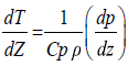
Mean seasonal tropospheric ozone partial pressure computed for the period 1998-2013 determines its mixing ratio in the atmosphere at a given altitude or barometric pressure (Table 2). As such, partial pressure measures the frequency of collisions of gas molecules with surfaces and therefore determines the exchange rate of molecules between the gas phase, and a coexistent condensed phase [38]. It is thus a useful parameter to determine dynamical and chemical properties of the troposphere as well as the tropopause characteristics. In this study, we use seasonal ozone partial pressure to determine stratospheric ozone exchange process which can be detected by ozone pressure lapse rate profile, which is expressed by the formula:
| Season | Ozone Partial pressure | Barometric Pressure inversion point (hPa) |
|---|---|---|
| DJF | 1 | 256 |
| MAM | 1.1 | 250 |
| JJA | 1.2 | 290 |
| SON | 1 | 261 |
Table 2: Seasonal ozone partial pressure inversion point variation as function of barometric pressure.
 (5)
(5)
Where T=air Temperature
z=Altitude
p=Atmospheric Pressure
cp=Caloric heat
ρ=air density
Suppose Q=Ozone partial pressure which change as function of atmospheric pressure, humidity and temperature, the following equation can be obtained:
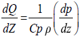 (6)
(6)
Figure 6 displays inversion lapse occurring at different atmospheric pressure values in all seasons. A remarkable inversion atmospheric pressure is noted in JJA and SON where ozone partial inversion profiles evolve at 298 hPa and 261 hPa in JJA and SON respectively and reach the highest value of 2.5 nm (nanometer) at 200 hPa considered at a tropopause pressure in the tropics. Therefore ozone partial pressure lapse rate increase as function of  implies stratospheric tropospheric ozone exchange between the upper troposphere and the lower atmosphere. This dynamic process is normally accompanied by strong radiative heating due to latent heat release at low latitude such as equatorial Africa. This change may spawn tremendous climate parameters change such as high surface temperatures with all the consequences that may follow in the region. Figure 7 present the seasonal ozone partial pressure inversion logarithmic model together with their respective regression coefficients R2. All seasons present a strong regression coefficient, which implies that STE activity occur in all seasons at Nairobi. Table 3 presents seasonal ozone partial pressure inversion variation at 200 hPa with equal value of 2.5 recorded in both winter and summer.

Figure 6: Mean seasonal tropospheric ozone and partial pressure at Nairobi for the period 1998-2013.

Figure 7A: Ozone partial pressure lapse rate for DJF Computation of seasonal ozone partial pressure profiles.

Figure 7B: Ozone partial pressure lapse rate for MAM.

Figure 7C: Ozone partial pressure lapse rate for JJA.

Figure 7D: Ozone partial pressure lapse rate for SON.
| Season | Barometric Pressure with high value (hPa) | Ozone Partial pressure |
|---|---|---|
| DJF | 200 | 1 |
| MAM | 200 | 1.8 |
| JJA | 200 | 2.5 |
| SON | 200 | 2.5 |
Table 3: Seasonal ozone partial pressure inversion variation at 200 hPa.
Computation of inter annual ozone concentration shows that high tropospheric ozone concentrations of 68 DU were recorded in July 2001 and October 2002 respectively. In order to understand the mechanisms responsible for these high ozone concentration events two case studies have been chosen and analysed. The ozone profile events on 25 July 2001 and on 09 October 2002 have been chosen as profiles presenting the highest ozone concentrations event of 126 ppbv at 100 hPa, and 121 ppbv at the same altitude (Figure 8).

Figure 8A: Tropospheric ozone profile with corresponding relative humidity at Nairobi 25 July 2001.

Figure 8B: Tropospheric ozone profile with corresponding relative humidity at Nairobi 9 October 2002.
Back trajectory computation from HYSPLIT trajectory Model has been used to determine the air mass trajectory that may have contributed to ozone enhancement events at Nairobi. Composite 24 hours trajectory modeled at three different altitudes, i.e. 3 000 m, 5 000 m and 7 000 m above ground level and at 8000 m, 10,000 m and 12,000 m were chosen with isobaric vertical motion. Two plots for individual event have been computed, and the results are presented in (Figure 9 and Figure 12). Mean eddy divergence plot have together with potential vorticity have been used to determine STE contribution to high ozone events on the days.

Figure 9A: Composite HYSPLIT back trajectory representing the air mass pathway at three different altitude 3000 m, 5000 m and 7000 m over Nairobi on 25/07/200 [41].

Figure 9B: Composite HYSPLIT back trajectory representing the air mass pathway at three different altitude 8000 m, 10000 m and 12000 m over Nairobi on 25/07/2001 [41].

Figure 10: Mean Eddy divergence average over June and July 2001 [42].

Figure 11: Vorticity Mean eddy vorticity June-July 2001 [42].

Figure 12A: Composite HYSPLIT back trajectory representing the air mass pathway at three different altitude 3000 m, 5000 m and 7000 m over Nairobi on 9/10/2002 [41].

Figure 12B: Composite HYSPLIT back trajectory representing the air mass pathway at three different altitude 6000 m, 10000 m and 14000 mm over Nairobi on 9/10/2002 [41].
Case study of 25/07/2001
Analysis of 25/07/2001 tropospheric ozone and relative humidity profiles (Figure 8a), shows two ozone peaks occurring at lower troposphere with 57 ppbv at 590 hPa and in the upper troposphere 126 ppbv at 100 hPa. These peaks are well in line with the findings made by Mulumba et al. (2015) on the positive correlation between ozone and relative humidity at surface and upper troposphere.
Surface to middle altitude display a decrease on ozone concentration value below 50 ppbv showing the minor photochemical sources contribution from local sources as shown in Figure 9a, at the altitude 3000 m, 5000 m and 7000 m. Photochemical contribution from neighboring Somalia can be observed at 350 hPa in the upper troposphere. The possibility of photochemical sources contribution cannot be excluded at this time of the year when north east monsoon prevail during the low sun season. However, the work done by Bundi et al. [10] evidenced ozone enhancement episodes over equatorial and southern Africa at mid–troposphere at locations distant from potential precursor source regions. These findings may be in agreement with approach developed by Holton et al. [39], on STE contribution to lower levels ozone these regions.
Figure 9b, plotted at the altitude of 8000 m, 10000 m and 12000 m clearly shows aim mass trajectory from Somalia from a distance as far as 700 km away from Nairobi. Local contribution of ozone enhancement on this day is from convective air mass driven by easterly flows. These flows are motivated by the proximity of the Indian Ocean which plays a crucial role on synoptic weather system in eastern Africa. Further analysis on dynamic parameters through NCEP/NCAR Reanalysis model shows a positive mean eddy divergence values during the month of June to July 2001 (Figure 10). Evidence of high vorticity 1 sigma occurring over the same period has been also noted with positive value 1.5e to 2.5e (Figure 11).
STE process contribution can be depicted through the sharp increase of ozone that occurs at 153 hPa with a concentration of 36 ppbv to peak up at 124 ppbv at 100 hPa under diabatic condition such was determined by ozone pressure positive lapse rate.
Case study of 09/10/2002
Analysis of 09/10/2002 tropospheric ozone and relative humidity profiles (Figure 8b), shows two ozone peaks occurring at mid-troposphere with 108 ppbv at 400 hPa and in the upper troposphere 120 ppbv at 100 hPa.
Over this date a sharp relative peak is noted at 700 hPa, which corresponds to ozone value of 33 ppbv. Once more, this is in good agreement with the positive correlation existing between ozone and relative humidity. A substantial increase in ozone concentration noted below 700 hPa originates from local photochemical sources and long distance air mass transport driven my easterlies flow as shown in Figure 12a. Consequently, a remarkable decrease in relative humidity at the same pressure and below is also noted.
A second peak, which originates from 250 hPa with ozone concentration of 38 ppbv to reach 120 ppbv at 100 hPa, denotes a contribution from local and long range air mass transport from photochemical sources in the upper troposphere driven by coupled ocean-atmosphere-land interactions (Kinyoda, undated) as displayed in Figure 12b.
These findings clearly show the role played by Indian Ocean on the synoptic weather system in equatorial eastern Africa. Although photochemical sources contribution from long range transport of air mass from Indian Ocean from easterly jet stream in the upper troposphere, have been noted, the possibility of STE contribution during this period of the year at Nairobi cannot be excluded (Kinyoda).
Long term mean eddy divergence 1 sigma computed from NCEP reanalysis model provides evidence positive values higher than winter period, which vary from 1.5e to 4.5e (Figure 13). Positive values on one month mean eddy vorticity model computation from NCEP/NCAR reanalysis model have also been noted (Figure 14). These parameters confirm well the higher contribution of STE to ozone enhancement in equatorial east Africa during SON than during

Figure 13: Mean Eddy divergence average over September-October 2002 [43].

Figure 14: Vorticity Mean eddy vorticity September-October 2002 [42].
JJA. During this season, the influence of ENSO (El Nino, Southern Oscillation) and the Quasi Biennial Oscillation (QBO) occurring at Nairobi cannot be ignored [40].
Tropospheric ozone climatology over equatorial eastern Africa has been investigated with data from SHADOZ Network from Nairobi, which is a unique station in this part of the continent where a few in situ tropospheric ozone measurements exist. Its geographic position near the equator and a few distance from Indian Ocean makes Nairobi one of the most complex meteorogical system in the African continent. In this study, we provide a brief summary of previous work encompassing the main circulation features, in order to undertand the dynamic that governs the tropospheric ozone variation over this region. Locate in a region of high ozone enhancement, a study of ozone distribution and variation using long term ozone sonde data, may provide a comprehensible tropospheric ozone for the eastern african region where ozone data are scarce and its climatology not well understood. This is in essence the purpose of this study the following objectives: to compute seasonal and annual tropospheric ozone distribution and variation, to assess seasonal variation with regard to climate change parameters, to assess ozone parameters variation and to determine origin photochemical sources as well as dynamical factors contributing to its enhancement in the region, and finally to predict future scenario on ozone enhancement and its consequences in the region. The main future of this study reveal seasonal tropospheric ozone variation with two maxima occurring in JJA (43 DU) and SON (46.8 DU). Vertical distribution displays two ozone peaks occurring in the same period with 121 ppm and 126 ppbv at 100 hPa. Seasonal ozone partial pressure profiles present strong regression coefficient (0.81