Journal of Oceanography and Marine Research
Open Access
ISSN: 2572-3103
ISSN: 2572-3103
Review Article - (2024)Volume 12, Issue 2
Internal tides are formed by the barotropic (surface) tides moving stratified water over sudden bathymetric changes. These phenomenon present an important control on climate dynamics, through the carbon cycle and the general ocean circulation and biological productivity in shelf seas. Turbulence closure schemes are used to model the effect of turbulence in a one dimensional water column. They are based on traditional boundary layer theory, which suggest that mixing is a result of boundary stresses. However, these schemes have been shown to be weak in simulating mixing in stratified water columns.
Three dimensional turbulence resolving models, such as Large Eddy Simulations (LES) have recently been applied to coastal regions. They allow for a much better understanding of turbulent processes as they directly derive each turbulent quantity. However, they often cannot be utilised due to their high computational cost. Although in recent years they have been used to improve turbulence closure schemes to better capture turbulent effects.
Three dimensional regional ocean model used by the MET office, presently cannot resolve the effect of internal tides. Once these regional models are able to resolve the phenomenon of internal tides, they will need turbulence closure models to capture the spatially varying mixing they induce. This literature review is written for the purposes of an MSc thesis project which aims to use LES to ‘tune’ a turbulence closure scheme to better capture the effect of internal tides. This work will further the understanding in this new area of research.
Internal tides; Buoyancy frequency; Turbulent effects; Turbulence closure schemes
Internal waves of tidal frequency are termed internal tides. Internal tides are found both in the deep ocean and the shallow continental shelf seas. Although shelf seas only make up a small amount of the ocean’s surface (<7%), they are thought to be locations where most of the tidal energy is dissipated. As the surface tide travels in a stratified water column sudden changes in sea floor topography, such as the shelf break can cause a tidal frequency oscillation in the pycnocline. Recent studies have shown an enhanced level of shear produced by the internal wave field in Eastern North America, also the breaking of internal waves can contribute significantly to the vertical structure of the water column through inducing turbulence. The importance of these effects in vertical mixing is demonstrated by the studies done to parameterise their effects in models describing turbulence [1].
Fluxes of pertinent properties such as momentum, heat, salt and nutrients necessary for primary production are dependent upon the vertical mixing caused by shear instabilities within the pycnocline region. Especially for biological productivity, vertical mixing offers a control to the spatial and temporal distribution of phytoplankton within the water column and through controlling the flux of nutrients to the base of the thermocline, the subsurface chlorophyll maximum (Figure 1). Vertical mixing processes are also crucial in completing our understanding of the carbon cycle and thus climate change. Recent work has brought attention to the role of turbulence within shelf seas in Siberia acting as a control on the flux of CH4 to the atmosphere, highlighting the importance of turbulence in the fluxes of gasses between the sea and the atmosphere [2].

Figure 1: Profile of chlorophyll concentration and temperature showing the sub-Surface Chlorophyll Maximum (SCM).
Apart from internal tides and waves, shear can be induced within the pycnocline region via wind stress, these forces when balanced with surface heating and its associated stabilisation effects, present a picture of the water column structure in shelf sea regimes. Turbulence closure schemes are employed and implemented within regional ocean models, in order to model the effect of turbulence within the water column. These schemes through parameterization and quantification of turbulent fluxes offer insight into modelling turbulent fluxes. The crucial role of turbulence across the pycnocline region in biological productivity, through the distribution of certain key nutrients and the global carbon cycle, necessitates that these turbulence closure models accurately represent mixing across density interfaces.
Internal tides and turbulence
Internal tides are caused by the surface (barotropic) tide moving a stratified column of water over a depth discontinuity. In the case of deep water this takes place at sea mounts or ridges. More importantly, this also takes place at the shelf edge where the internal wave subsequently propagates as a mainly semidiurnal frequency (M2) thermocline oscillation. Although due to the non-linear effects of a sloping bottom topography (shelf seas), internal tides can also manifest as non-linear internal waves, exhibiting a higher frequency (10-30 minutes) then the semidiurnal. Internal waves generate turbulence which leads to mixing and studies have shown that this mixing is mostly a result of shear instabilities. Figure 2 shows that buoyancy frequency is lowest when sea floor topography exhibits drastic changes. A reduced buoyancy frequency is indicative of weak stratification and hence a relative increase in shear effects as outlined by the gradient Richardson’s number (Figures 2 and 3) [3].

Figure 2: Contours of buoyancy frequency (cph) as a function of latitude.

Figure 3: Schematic of tidal dissipation.
A study done in the western long island sound found that the internal waves disturb the thermocline, at times by perturbing the thermocline up to half the water depth. In the liverpool bay, looking at a Region of Freshwater Influence (ROFI), Simpson, et al. found that there is an asymmetry in terms of dissipation with heightened levels of dissipation and thus mixing, occurring at flood tide (Figure 4) [4].

Figure 4: a) Summer sea surface temperature for the North West European shelf seas, with labelled locations corresponding to positions of temperature profiles, b) The temperature profiles highlight the generally diffuse nature of the thermocline in shelf seas.
Turbulence closure
The principle of Turbulence Closure (TC) schemes is based on splitting the flow into a mean and a fluctuating component, otherwise known as Reynolds averaging. This allows for the definition for the total energy contained in turbulence or TKE. The existence of turbulence closure scheme stems from a need to relate the eddy parameters, which represent turbulence, to other system variables. This need can be fulfilled by either parameterising the turbulent quantities as a single value or by taking a more complex approach and assigning a number of equations to relate turbulent quantities to the other flow parameters [5].
Physical considerations of TC
The Navier stokes equations represent a single universal equation for describing turbulent effects. In the marine environment an appropriate approximation made is that proposed by Boussinesq. Through the use of the Reynolds decomposition, the Navier stokes equations can be rewritten, giving rise to time averaged equations describing fluid flow. The equation of TKE and its dissipation are properties of turbulence defined through the RANS equations. The Reynolds stresses as well as the turbulent fluxes of heat and salt comprise unknown second moments in the RANS equation [6].
Many closure schemes have been developed utilising two equations, the first equation often describes the progression of TKE donated by k, which is both produced and dissipated within the fluid flow (first and third terms on the RHS), as well as being altered through advection and diffusion processes (second equation on the LHS).
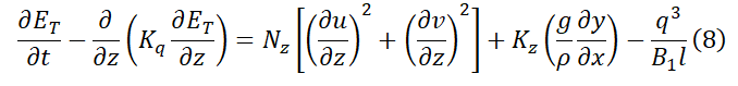
Figure 5 outlines the various models in existence which tackle turbulence closure in the ways outlined above.

Figure 5: The various statistical turbulence closure schemes.
The models discussed above have been shown to perform similarly when their buoyancy production is modified based on Burchard and Baumert (k-ε) and Burchard (k-kl).
Studies have found a variation in the diffusivity in shelf sea regions on both temporal and spatial time scales. If this nature of diffusivity is incorporated within the closure schemes it would allow for a more accurate representation of thermocline dissipation. In a way this has been addressed by a more recent study, which, through the application of three different background diffusivities to a turbulence closure scheme, Rippeth found that an adequate representation of thermocline dissipation, relative to observation of dissipation, can be established with a background diffusivity orders of magnitude greater than molecular diffusivity. However in light of the aforementioned nature of diffusivity, the methodology employed by Rippeth is called in to question [7].
Comparison with observation
Recent advances in technology have given rise to new ways in which the measurement of turbulence dissipation in shelf sea regions can be carried out. Although observations of turbulence suffer as many setbacks as turbulence closure schemes, they can offer valuable insight into the performance of turbulence closure schemes in modelling turbulent mixing.
Studies done on variants of the Mellor Yamada closure schemes and observations of turbulence taken by a fly profiler in the Irish sea (Figure 6). Simpson et al compared TC models to observations of turbulence, in the form of dissipation profiles at both stratified and mixed regimes in the Irish sea. The data gathered was plotted as a profile of log10ε (dissipation) (Figures 7 and 8) [8].

Figure 6: Map of the Irish sea.
Simulated and observed dissipation profiles differed significantly in the stratified regime (S1) (Figure 8). From the approximation made for the MY 2.2A, in which the eddy diffusivity were set equal to the eddy viscosity, thermocline dissipation in the interior of the water column was underestimated by approximately four orders of magnitude (Figure 9b), relative to observation.
This result, along with the good replication of the observed dissipation profile in the well mixed regimes, leads to the conclusion that there is an additional source of TKE within the interior of the water column, as MY 2.2 A and B account for the vertical diffusion of TKE by boundary layer stresses. An interior source of turbulence as found by Rippeth and Green, et al. is thus inadequately represented using traditional boundary layer theory, as utilised by the MY closure schemes [9].

Figure 7: Profiles of dissipation (log10ε) in Wm-2 taken from the mixed location M1 over two tidal cycles. Observed levels of dissipation as measured using a FLY profiler (a) and modelled using MY2.2A and MY2.0.

Figure 8: Temperature profile (°C) as measured in the stratified location, S1 (a) Observed levels of dissipation collected using the fly profiler from the stratified location (S1) and modelled by the MY2.2B (c) and MY2.0 (d). The profiles were taken over two tidal cycles.

Figure 9: Modelled profiles of dissipation, in both the well-mixed M3 location (a) and stratified S1 location (b).
This shows a seemingly inherent inability of statistical turbulence closure schemes in accurately assessing mixing along the pycnocline. The fact that the closure schemes showed a good representation of turbulent dissipation in well mixed regimes and not stratified regimes, leads one to conclude that there may be a source of TKE produced in the pycnocline region [10].
Turbulence resolving models
LES provide a unique opportunity in trying to improve the performance of statistical turbulence closure models via giving insight into turbulent effects leading to the parameterisation of ‘missing’ effects in the 1d closure schemes. LES studies have been applied successfully to the atmosphere, leading to the advancement of the Mellor Yamada model, as well as the parameterization of LC in second moment closure models.
LES employ a filtered form of the Navier stokes equation. This results in terms describing sub grid turbulent processes. For these reasons, grid and time-step requirements result in LES being computationally expensive [11].
Although there use has typically been focused on the deep ocean, with the use of open bottom boundary conditions, recent work has applied LES to coastal regions. Burchard et al, applied LES to coastal regions by defining a shallow water column forced by wind stress (0.1 Nm-1) and the presence of a wave field (30 m wavelength and a significant wave height of 1 m), at the surface, ignoring the effect of stratification. They found that, after the model was run for 2 h, due to the surface wave forcing, LC were evident throughout the flow, with depth varying scales (Figure 10) [12].

Figure 10: LES model run for the case of a well-mixed, shallow water column.
Burchard, et al. also ran the model for the same duration for a stratified water column in the presence of a topographical feature, which represented an obstacle to the flow. The movement of stratified water over an obstacle can generate internal waves, as previously discussed. Out of the parameters which are used to quantify this response, the mode number of internal waves is the most pertinent. It is related to the buoyancy frequency (1), the water depth (H) and the velocity over the feature (obstacle) and quantifies the number of wave components over the obstacle. When two components of the wave are evident, pycnocline structure is more variable (Figure 11 b), relative to the large thermocline oscillations in the presence of a single wave component (Figure 11 a).

Figure 11: LES run for a stratified shallow water column in the presence of obstacle.
3d models such as NEMO incorporate turbulence closure schemes in order to model vertical mixing. Therefore, it is of priority to accurately parameterise interior mixing effects in these 1d models and studies, such as those carried out by Kantha and Clayson, Gregg, Kunze, et al. and Mackinnon and Gregg, have attempted to do this very thing. Research done by Simpson, et al. on the Mellor Yamada closure schemes, showed that the model underestimated mixing effects in the interior of the water column in a stratified regime by approximately 4 orders of magnitude. However in a well-mixed regime when vertical diffusivity was allowed, the model accurately characterised mixing effects throughout the water column, relative to observational data. the traditional boundary layer theory, which presumes stresses are solely from the surface and bottom boundary layers, employed by turbulence closure schemes is in sufficient given that there has been shown to be an interior source of TKE.
Large eddy simulation, through solving for each turbulent quantity, can be used as a way of measuring the capabilities of turbulence closure models to resolve turbulent processes. They have also been shown to provide a way of improving turbulence closure models by paving a way to the parameterisation of certain effects. However due to the high computational cost of LES, as they have fine grid resolutions, they often cannot be utilized.
Citation: Piracha A (2024) Turbulance Closure Models. J Oceanogr Mar Res. 12:304.
Received: 21-Oct-2019, Manuscript No. OCN-24-2531; Editor assigned: 24-Oct-2019, Pre QC No. OCN-24-2531 (PQ); Reviewed: 07-Nov-2019, QC No. OCN-24-2531; Revised: 31-May-2024, Manuscript No. OCN-24-2531 (R); Published: 28-Jun-2024 , DOI: 10.35248/2572-3103.24.12.304
Copyright: © 2024 Piracha A. This is an open-access article distributed under the terms of the Creative Commons Attribution License, which permits unrestricted use, distribution, and reproduction in any medium, provided the original author and source are credited.