Journal of Aeronautics & Aerospace Engineering
Open Access
ISSN: 2168-9792
ISSN: 2168-9792
Research Article - (2015) Volume 4, Issue 2
Analytical solutions with the KS element equations of motion due to the combined effect of zonal harmonics J2,J3 and J4 and drag by considering an analytical oblate diurnal exponential density model when density scale height varies with altitude is obtained using series expansion method. Terms up to third terms in e, eccentricity, c, a small parameter depending on the ellipticity of the atmosphere and second order terms in μ, gradient of the scale height altitude are considered. The KS element equations are numerically integrated (NUM) through a fixed step size fourth-order Runge-Kutta-Gill method having a very small step-size of half degree in the eccentric anomaly for comparing analytically integrated (ANAL) values. After 100 revolutions, decrease in argument of perigee, ω, at perigee height = 400 kilometer, e = 0.1 and inclination i = 20 and 80 degrees, are found to be 7.42 and 39.8 degrees. At i =80 degree, the percentage error = (ANAL - NUM) / NUM after 1 and 100 revolutions are 0.61 and 2.09.
<Keywords: Ks elements; Zonal harmonics; Atmospheric drag; Analytic integration
The dynamical system of a satellite motion perturbed by both atmospheric drag and gravitational attraction is nonlinear, non conservative in form and the integration of the system, in general, is analytically intractable. To predict the motion precisely a mathematical representation for these forces must be selected for integrating the resulting differential equations of motion. Some of the early studies and analytical difficulties for the coupled problem were addressed by de Nike [1]. Hoots [2] used the gravitational and atmospheric models as used by Lane [3] and arrived at an improved analytical solution. Well known and commonly used models [4-9]. The KS total-energy elements equations [10] is a very powerful method for numerical solution with respect to any type of perturbing forces as the equations are less sensitive to round-off and truncation errors in the numerical integration algorithm. Sharma worked with these KS element equations to compute very accurate short-periodic terms due to J2, even for very high eccentricity orbits [11,12]. Sharma [13,14] expanded analytic solutions by series expansion method using analytical models for oblate exponential atmospheric density model, and a model of the same with the effect of diurnal bulge.
In this paper my attempt is to get analytical solutions with the KS element equations of motion for long-term motion by considering the perturbations due to the combined effect of Earth’s zonal harmonics J2 to J4 and atmospheric drag. The model used here is an oblate diurnally varying atmosphere with variation of the scale height depending on altitude almost similar to my work with Sharma [15]. Using series expansion method third-order terms in e, eccentricity, c, a small parameter depending on the ellipticity of the atmosphere and second order terms in μ, gradient of the scale height altitude are collected. Only one of the eight equations is solved analytically to obtain the state vector at the end of each revolution due to symmetry in KS equations. Numerical studies with test cases reveal that there is a good comparison between the analytical (ANAL) and numerically integrated (NUM) values of the position as well as velocity vectors  and
and  .
.
The KS element equations of motion of a satellite under the effect of perturbing potential V and additional perturbing force  [10] are
 (1)
(1)
 (2)
(2)
 (3)
(3)
 (4)
(4)
 , specifying attraction between two masses M and m, E, ω,t,r and k2 are, respectively,the eccentric anomaly, angular frequency, physical time, radial distance and the gravitational constant.
The perturbing potential V[10] and the aerodynamic drag force  [16] per unit mass acting on a satellite of mass m are respectively
 (5)
(5)
R, equatorial radius, Jn ’s, dimensionless constants known as zonal harmonics. Using Equation (5),
where

As in [16],  the effective area of the satellite, CD, the drag coefficient, ρ , the atmospheric density at the point of calculating atmospheric drag force and
  , the velocity of the satellite relative to the ambient air. If
  is the velocity of the satellite relative to the Earth’s centre, then
  where
where  is the velocity of the air relative to the Earth’s centre is assumed to be west to east,
  Λ ,the rotational rate of the atmosphere about the Earth’s axis and i0, the initial inclination,
  is the initial perigee radius,
  the velocity at the initial perigee. Then the drag force per unit mass tangential to the orbit can be written as
 Where
Where  and
and
 (6)
(6)
Following [17] the density function for an oblateness atmosphere together with day-to-night density variation is
 (7)
(7)
To express cosφ in terms of the true anomaly θ and then in terms of the eccentric anomaly E let  and
and  are the right ascension and declination of the sun and the day time bulge respectively, then
 . We can write
 (8)
(8)
 (9)
(9)
 (10)
(10)
The scale height H is known to increase with altitude and this variation of H will have an influence upon its motion. The value of H may be taken as  =where |μ |< 0.2 and for any particular value of rp. To sum up, expression for the density, similar to that of Swinerd Boulton [17], is
 (11)
(11)


In terms of E,
 (12)
(12)
 (13)
(13)
 (14)
(14)
The integrals available in the above theory are of the form
 and 0 if either m or n is odd.
Knowing the position and velocity vectors and at the instant t = 0 , the values of  and
and  can be computed [10], (pp. 91-92), and by adopting E = 0 as the initial value of the eccentric anomaly, we obtain
In the entire test cases reported here, the values of ω , Right Ascension Node, Ω and mean anomaly, M are 60, 30 and 0 degrees respectively. The value of K2, R, J2, J3 and J4 utilized for numerical computations are 398600.8km3s−2 , 6378.135 kilometer and  ,−2.53648D − 06 and -1.52D-06 respectively. Jacchia (1977) atmospheric density model, which is relatively easier to use, is employed to compute the values of ρp0 , the density at the perigee and H, the density scale height at the end of each revolution. Arbitrarily 22 August 2002 is chosen as the initial epoch. The values of ε, ∧ and
  , utilized during the computations are 0.00335, 1.2 and 50.0 respectively. In this model
  sin i approaches maximum value 0.2042 at e = 0.003 and i= 80° while minimum value 0.0232 at e = 0.005 and i= 20° respectively at the end of 100 revolutions (Figures 1 and 2). The values of 10.7cm solar flux (F10.7) and averaged geomagnetic index (AP) are taken as 150 and 10, respectively, which approximately represents an average density and results in exospheric temperatures between 1000 and 1100 K for the different cases we considered (Table 1).
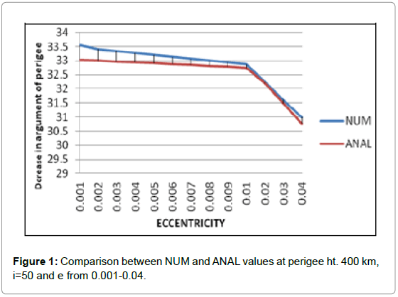
Figure 1: Comparison between NUM and ANAL values at perigee ht. 400 km, i=50 and e from 0.001-0.04.
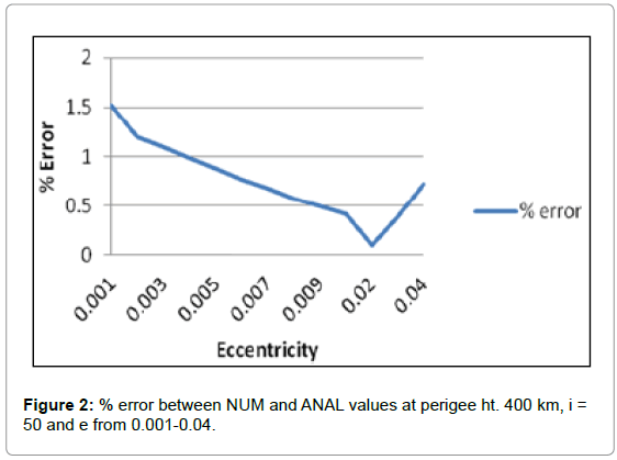
Figure 2: % error between NUM and ANAL values at perigee ht. 400 km, i = 50 and e from 0.001-0.04.
| Perigee heights in Km | |||||||
|---|---|---|---|---|---|---|---|
| e | Method | 350 Inclination in Degrees | 400 | ||||
| 20 | 50 | 80 | 20 | 50 | 80 | ||
| 0.003 | NUM | 49.658 | 33.851 | 9.213 | 48.891 | 33.336 | 9.069 |
| ANAL | 49.185 | 33.585 | 9.181 | 48.416 | 32.971 | 8.884 | |
| % ERROR | 0.95 | 0.79 | 0.35 | 0.97 | 1.1 | 2.04 | |
| 0.004 | NUM | 49.561 | 33.783 | 9.193 | 48.796 | 33.269 | 9.05 |
| ANAL | 49.104 | 33.584 | 9.156 | 48.327 | 32.942 | 8.866 | |
| % ERROR | 0.92 | 0.59 | 0.4 | 0.96 | 0.99 | 2.04 | |
| 0.005 | NUM | 49.463 | 33.715 | 9.173 | 48.7 | 33.203 | 9.032 |
| ANAL | 49.017 | 33.582 | 9.115 | 48.236 | 32.912 | 8.852 | |
| % ERROR | 0.9 | 0.39 | 0.64 | 0.95 | 0.88 | 1.99 | |
| 0.007 | NUM | 49.2681 | 33.58 | 9.137 | 48.507 | 33.071 | 9 |
| ANAL | 48.832 | 33.57 | 9.063 | 48.049 | 32.849 | 8.833 | |
| % ERROR | 0.89 | 0.03 | 0.8 | 0.94 | 0.67 | 1.81 | |
| 0.008 | NUM | 49.171 | 33.513 | 9.118 | 48.411 | 33.005 | 8.978 |
| ANAL | 48.734 | 33.558 | 9.039 | 47.953 | 32.814 | 8.825 | |
| % ERROR | 0.89 | 0.13 | 0.87 | 0.95 | 0.58 | 1.71 | |
| 0.009 | NUM | 49.073 | 33.447 | 9.1 | 48.316 | 32.939 | 8.96 |
| ANAL | 48.633 | 33.542 | 9.024 | 47.857 | 32.777 | 8.817 | |
| % ERROR | 0.9 | 0.28 | 0.84 | 0.945 | 0.49 | 1.6 | |
Table 1: Decrease in Argument of Perigee.
We have transformed equations for  and using equations (11), (12), (13), (14) and programmed in double precision arithmetic to compute the KS elements
  and
and  (i = 1,2,3,4). Once and are known, they are converted into and and , which are further converted to the osculating orbital elements (Figures 3 and 4). Percentage Error = (ANAL – NUM)/NUM is calculated to check validity of the work. The algebraic computations are made with MAPLE12 mathematical software (Table 2).
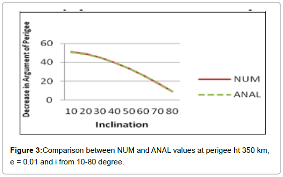
Figure 3: Comparison between NUM and ANAL values at perigee ht 350 km, e = 0.01 and i from 10-80 degree.
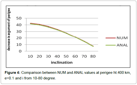
Figure 4: Comparison between NUM and ANAL values at perigee ht.400 km, e=0.1 and i from 10-80 degree.
| e | After 1 revolution | After 100 revolutions | ||||
|---|---|---|---|---|---|---|
| NUM | ANAL | % error | NUM | ANAL | % error | |
| 0.01 | 0.5029 | 0.5019 | 0.2 | 48.2202 | 47.7593 | 0.96 |
| 0.02 | 0.4931 | 0.4919 | 0.24 | 47.2798 | 46.7755 | 1.07 |
| 0.03 | 0.4835 | 0.4822 | 0.28 | 46.3662 | 45.8329 | 1.15 |
| 0.04 | 0.4743 | 0.4728 | 0.32 | 45.4785 | 44.9364 | 1.19 |
| 0.05 | 0.4653 | 0.4636 | 0.36 | 44.616 | 44.0643 | 1.24 |
| 0.06 | 0.4566 | 0.4548 | 0.4 | 43.7776 | 43.2031 | 1.31 |
| 0.07 | 0.4481 | 0.4461 | 0.44 | 42.9625 | 42.3474 | 1.43 |
| 0.08 | 0.4398 | 0.4377 | 0.49 | 42.1698 | 41.4952 | 1.6 |
| 0.09 | 0.4318 | 0.4295 | 0.55 | 41.3988 | 40.6458 | 1.82 |
| 0.10 | 0.424 | 0.4214 | 0.61 | 40.6485 | 39.7981 | 2.09 |
Table 2: Comparison of ANAL to NUM with % error at perigee ht 400 km, i = 80 after 1and 100 revolutions.
The KS element equations are integrated analytically by a series expansion method by assuming an oblate diurnal atmosphere when density scale height varies with altitude and by including the terms corresponds to Earth’s zonal harmonics J2, J3 and J4. A wide range of eccentricity and inclination is considered for calculating the change in argument of perigee by present analytical theory and by numerical integration. Comparison between analytically and numerically integrated values for 1 and 100 revolutions shows that the analytically integrated values are reasonably accurate and thus highlights the usefulness of the analytical expressions. Graphical representation as well as the table presented here emphasizes the importance of developing the theory to find the decrease in argument of perigee.